Unifying machine learning and interpolation theory via interpolating neural networks

Emerging scientific computational methods are moving from relying on explicitly defined and modular programming to the adoption of neural network-based self-corrective algorithms. In computer science, this transition is coined as “from Software 1.0 to Software 2.0”¹. The shift towards software 2.0 partially resolves the issue of labor-intensive programming in Software 1.0 and has significantly advanced the domain of large language models (LLMs) and other foundational models^2,3. However, adopting a similar technology in the fields of computational engineering and science presents unique challenges: generality, data-hunger, scalability, and sustainability. Machine learning (ML)-based partial differential equation (PDE) solvers do not generalize with the same level of accuracy as traditional numerical methods^4,5,6,7,8. Hence, researchers are cautiously re-evaluating the effectiveness of the ML-based PDE solvers^8,9. The success of purely data-driven ML models on sparse datasets is always limited¹⁰. The scalability of the neural network-based solver is of major concern when dealing with extremely high-dimensional inverse system design. High-fidelity numerical methods with over millions of degrees of freedom (DoFs) are often required for simulating the additive manufacturing (AM) process or integrated circuit (IC) at extremely fine resolution and multi-physics/multiscale setup^11,12,13. Furthermore, the solution is often unusable for different materials or processing scenarios and requires repeated solutions of extremely large systems. Finally, the energy cost associated with very large-scale ML models is becoming prohibitive. The energy consumption required to train the largest ML models increased by six orders of magnitude from 2012 to 2018¹⁴, and there are growing concerns about fresh water consumption for cooling massive AI data centers¹⁵. Hence, the sustainability of this new generation of computational tools will become a major concern.

In this context, this paper introduces an Interpolating Neural Network (INN), a computational framework for constructing machine learning models that emulate the behavior of PDE solvers, such as the finite element method (FEM)^16,17,18, and a purely data-driven tool, such as deep neural networks (DNNs) with the same architecture. The development of INNs was inspired by the hierarchical deep-learning neural network (HiDeNN) framework and its variants^{7,17,18,19,20,21,22}, which were originally designed for solving PDEs. INNs build on this foundation by reinterpreting components of numerical analysis as machine learning parameters, thereby generalizing their use for training, calibration, and the solution of various scientific and engineering problems. The goal of an INN is to create generalizable, transferable, scalable, and sustainable tools for the next generation of engineering software.

Curiously, although FEM and DNNs have different origins and purposes, they share one thing in common: they approximate functions. The former approximates a function with interpolation functions (or shape functions—the frequently used terminology in FEM) generated from discrete nodal coordinates in the input domain and with the corresponding nodal values in the output domain, while the latter constructs a black-box function space using neural networks parameterized with weights, biases, and activation functions. Nevertheless, it is possible to view a DNN as a general case of interpolation-based methods, such as FEM where the nodes are shifted from space-time input domain to a more general input domain that can comprise any quantity (word embeddings, pixel values, etc.), interconnectivity of FEM nodes is expressed as computational graph (connectivity in graph-based networks), and interpolation functions act as the nonlinear activation functions.

On top of this, separating each input parameter dimension with tensor decomposition (TD)^19,20,21,23 can make INNs scalable. Since the interpolation functions are interpretable and adaptable (i.e., one can adjust the basis functions that construct interpolation functions), and TD is scalable, INNs fuse these ideas to create accurate and sustainable computational tools.

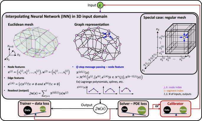
INNs follow three steps: 1) discretize an input domain into non-overlapping segments whose bounds are denoted by interpolation nodes, 2) construct a computational graph with the interpolation nodes, and formulate interpolation functions similar to message passing operations in graph-based neural networks^24,25,26, and 3) optimize the values and coordinates of the interpolation nodes for a given loss function. Figure 1 illustrates the approach in the 3D input domain. When the input domain is discretized with a regular mesh (see the special case in Fig. 1), INNs leverage TD to convert the growth rate of the computational cost to the problem dimension from exponential to linear. INNs are very flexible in performing 1) data training, 2) PDE solving, or 3) parameter calibration while using the same architecture. The computer codes can be found at https://github.com/hachanook/pyinn.

The INN box illustrates the graph representation of the input domain discretized with an arbitrary Euclidean mesh (left) and a regular mesh as a special case (right). Node and edge features are given from the mesh. After Q-step message passing, each node j will store an interpolation function N^[Q](j)(x). Finally, the readout operation sums the product of the interpolation functions N^[Q](j)(x) and nodal values u^(j). The superscripts with square brackets [] and parentheses () denote the message passing step and graph node index, respectively. The interpolation operator ({{mathcal{J}}}) denotes that ({{mathcal{J}}}{{boldsymbol{u}}}({{boldsymbol{x}}})) is a function that interpolates discrete values of u^(j). The INN trainer employs data-driven loss functions (e.g., mean squared error loss for regression), while the INN solver adopts a residual loss of a partial differential equation (PDE). A trained/solved INN model can then be employed as a forward model of a calibrator to solve an inverse problem.

Full size image

This article discusses the details of constructing an INN and implementing it to solve several benchmark problems in a purely data-driven setting, and solving both forward and inverse problems when a PDE is known. As a demonstrative engineering application of INNs, a simulation of process variation in laser powder bed fusion (L-PBF) AM is considered. In L-PBF, a laser is used to melt and fuse layers of metal powders to build a metal component. As the laser spot size ranges from 50 to 100 μm^11,27, physical simulations of AM require a sub-10-micron resolution that challenges most traditional numerical methods^12,28. The required computational resources become prohibitive, particularly when they are employed to generate training data for a surrogate model within a vast parametric space. As illustrated in Fig. 2, the INN presents a new direction toward part-scale AM simulations for online manufacturing control, demonstrating performance gains by orders of magnitude. The article also conducts various numerical experiments that cover computer science and engineering domains to demonstrate the superior capabilities of INNs in training, solving, and calibrating.

Detailed problem definition and explanation can be found in the Discussion section. We compare the single-scale finite-difference method (FDM) solver²⁸, the variational multiscale FEM solver¹², and the INN solver with CANDECOMP/PARAFAC (CP) decomposition and Q = 2. The data points for the first two methods with dashed marker edges are estimated as they are intractable with a single GPU, while those of INN with a solid marker edge are computed. All benchmarks were conducted with a single GPU, NVIDIA RTX A6000 GPU with 48 GB VRAM.

Full size image

Discretization of the input domain

Consider a regression problem that relates I inputs and L outputs. The first step of an INN is to discretize the input domain in the I-dimensional Euclidean space into a mesh, which can be as general as an unstructured irregular mesh or as specific as a structured regular mesh. In any case, a mesh in the Euclidean space can be readily represented as a graph—the most general form of a discretized input—as illustrated in Fig. 1. The graph nodes in an INN are arbitrary points in the input domain, which are irrelevant to the data structure. This is a key distinction of an INN from the graph neural network (GNN), which will be elaborated upon in the following discussion.

Suppose there are J nodes (or vertices) and E edges in the graph, where the input domain is discretized with C non-overlapping segments. Each segment occupies a subspace of the I-dimensional input domain. Each node (e.g., node j) has features: nodal coordinates (({{{boldsymbol{x}}}}^{(j)}in {{mathbb{R}}}^{I})) and values (({{{boldsymbol{u}}}}^{(j)}in {{mathbb{R}}}^{L})). The superscript with parentheses refers to the graph node index. An edge that links node j and k has a feature e^(j, k) that stores indices of segments connected to the edge. For example, when I = 3, L = 2, node 10 in Fig. 1 stores ({{{boldsymbol{x}}}}^{(10)}=({x}_{1}^{(10)},{x}_{2}^{(10)},{x}_{3}^{(10)})) and ({{{boldsymbol{u}}}}^{(10)}=({u}_{1}^{(10)},{u}_{2}^{(10)})). The edge connecting nodes 30 and 12 stores e^(30, 12) = {5, 7}.

Construction of INN interpolation functions via message passing

Once the input domain is properly discretized, INN message passing is conducted to build an interpolation function on each graph node. A typical message passing in a graph-based neural network returns a hidden state for each graph node, which is essentially a tensor (including matrix and vector)²⁴. In contrast, the INN message passing returns a function (i.e., interpolation function N^(j)(x), or often called shape function in FEM) for each node (j = 1, …, J) as a hidden state. A general Q-step message passing of an INN, ({{{mathcal{M}}}}^{[q]}(*)), can be expressed as:

where ({{{mathcal{N}}}}^{s}(j)) is a set of neighboring nodes of the center node j with s connections (i.e., s-hops, see Fig. 3 and Supplementary Information (SI) Section 1.1 for high-dimensional cases). The operation ({{{mathcal{M}}}}^{[q]}(*)) constructs an interpolation function N^[q](j)(x) for a graph node x^(j) using neighboring nodal coordinates and edge information, x^(k), e^(j, k), and the interpolation function of the previous message passing, N^[q−1](j)(x).

The function N^[Q](j)(x) is the INN interpolation function at node j after Q message passing. The ({{{mathcal{N}}}}^{s}(j)) is a set of neighboring nodes of the center node j with s connections (or s-hops).

Full size image

It is worth noting that the interpolation functions used throughout this article satisfy the Kronecker delta property, i.e., N^[q](j)(x^(k)) = δ_jk, meaning that the INN function space exactly passes the interpolation points. However, this condition may be relaxed depending on the specific problem and the chosen interpolation method. For instance, if the training data is highly noisy or spline basis functions are used, this condition may no longer be necessary.

With a single message passing (Q = 1) and s = 1 hop, the INN message passing degenerates to the standard FEM linear shape function (or Lagrange polynomials of order P = 1). As illustrated in Fig. 3 (left), it is the most localized approximation of an INN. In this case, the message passing operation at node j = 3 is written as:

where A^(c) refers to the region of segment c; e.g,. A⁽²⁾ = [x∣x⁽²⁾ ≤ x ≤ x⁽³⁾].

One can progressively enlarge the support domain and the approximation capability of an interpolation function by adding message passing with a higher hop. For instance, the second message passing with s = 2 hop constructs compact-supported interpolation functions with higher nonlinearity. This is theoretically equivalent to the generalized finite element method (GFEM)²⁹ and convolution hierarchical deep-learning neural networks (C-HiDeNN)^7,20. The message passing with a max-hop (Fig. 3, right) can even make it a non-local approximation where the support of interpolation functions occupies the entire input domain, mimicking meshfree methods that exhibit superconvergence (i.e., faster convergence rate than the complete order of polynomial basis)^30,31,32. Depending on the choice of interpolation technique, other hyperparameters can be involved in ({{{mathcal{M}}}}^{[q]}(*)), such as the activation (or basis) function and dilation parameter^7,20. This enables adaptive update of INN interpolation functions during training to improve accuracy (see SI Section 2.2). A more comprehensive discussion on functional approximation through interpolation theory and subsequent solvers can be found in refs. ^33,34,35. See SI Section 1 for various choices of the message passing operation.

Regardless of the choice of interpolation technique for the message passing, the global DoFs (i.e., number of nodes) remain constant. INNs adapt nodal connectivity through the adjacency matrix and basis functions to reproduce almost any interpolation technique available in numerical methods. The compact-supported interpolation functions enable INNs to be optimized locally and promptly, making INNs distinguishable from MLPs. Since an MLP is a global approximator, INNs with compact-supported interpolation functions 1) converge faster than MLPs with the same number of trainable parameters, and 2) facilitate training on a sparse dataset.

INN forward pass

During the forward propagation, an input variable ({{boldsymbol{x}}}in {{mathbb{R}}}^{I}) enters each graph node’s interpolation function N^[Q](j)(x), followed by a graph-level readout operation:

where the superscript [Q] is dropped for brevity (i.e., N^[Q](j)(x) = N^(j)(x)). The interpolation operator ({{mathcal{J}}}) will designate an interpolated field output throughout this paper. The readout operation can be written as a matrix multiplication:

where ({{{boldsymbol{u}}}}^{(j)}in {{mathbb{R}}}^{L},{{boldsymbol{U}}}in {{mathbb{R}}}^{Ltimes J},{{bf{{{mathcal{X}}}}}}(x)in {{mathbb{R}}}^{J}). The matrix U is a horizontal stack of nodal values u^(j), while ({{bf{{{mathcal{X}}}}}}(x)) is a vectorized function of x that is parameterized with nodal coordinates x^(j) during the message passing operation.

The graph node features (i.e., coordinate (x^(j)) and value (u^(j))) are trainable parameters of the INN. If the nodal coordinates (x^(j)) are fixed, one can find nodal values (u^(j)) without changing the discretization of the input domain. If the nodal coordinates are also updated, the optimization will adjust the domain discretization similar to r-adaptivity in FEM^17,18. Once the forward propagation is defined, the loss function is chosen based on the problem type: training, solving, or calibrating (see Method Section for details).

TD for model order reduction and scalability

When the input domain is discretized with a regular mesh, as illustrated in the special case of Fig. 1, we can significantly reduce the trainable parameters (or degrees of freedom, DoFs) by leveraging TD²³ that makes INN scalable. Here, we introduce the two widely accepted TD methods: Tucker decomposition^36,37 and CANDECOMP/PARAFAC (CP) decomposition^38,39,40.

One of the widely used TD methods is Tucker decomposition^36,37. It approximates a high-order tensor with J_i nodes in i-th dimension as a tensor contraction between dimension-wise matrices and a core tensor ({{bf{{{mathcal{G}}}}}}), which has the same order of the original tensor but with smaller nodes M_i (<J_i). The M_i is often called a “mode” to distinguish it from the original node J_i.

Consider a three-input (I = 3) and one output (L = 1) system, and assume the input domain is discretized with J = J₁ × J₂ × J₃ nodes, as shown in the special case box of Fig. 1. To facilitate tensor notation, the nodal values will be denoted with left/right super/sub scripts, (begin{array}{l}m\ iend{array}{u}_{l}^{(j)}), where (iin {{mathbb{N}}}^{I}) is the input index, (min {{mathbb{N}}}^{{M}_{i}}) is the mode index, (lin {{mathbb{N}}}^{L}) is the output index, and (jin {{mathbb{N}}}^{{J}_{i}}) is the nodal index.

The interpolated field ({{mathcal{J}}}u({{boldsymbol{x}}})in {{mathbb{R}}}^{L=1}) can be represented as a Tucker product:

where the core tensor ({{bf{{{mathcal{G}}}}}}in {{mathbb{R}}}^{{M}_{1}times {M}_{2}times {M}_{3}}) is a trainable full matrix typically smaller than the original tensor that compresses the data. Here, ({{bf{{{mathcal{A}}}}}}{times }_{a}^{b}{{bf{{{mathcal{B}}}}}}) denotes the tensor contraction operation between the a-th dimension of tensor ({{bf{{{mathcal{A}}}}}}) and the b-th dimension of tensor ({{bf{{{mathcal{B}}}}}}). The ({{mathcal{J}}}begin{array}{l}\ iend{array}{{boldsymbol{u}}}({x}_{i})in {{mathbb{R}}}^{{M}_{i}times 1}) is one-dimensional (1D) interpolated output of ith input dimension over M_i modes represented as:

where (begin{array}{l}\ iend{array}{{boldsymbol{U}}}in {{mathbb{R}}}^{{M}_{i}times {J}_{i}}) and (begin{array}{l}\ iend{array}{{bf{{{mathcal{X}}}}}}(x)in {{mathbb{R}}}^{{J}_{i}}). As illustrated in the special case box of Fig. 1, the message passing (blue arrow) only happens in the axial directions, yielding 1D interpolation functions: ({N}^{({J}_{i})}({x}_{i})).

When there is more than one output (L > 1), the interpolated field becomes a vector of L elements:

where ({{mathcal{J}}}begin{array}{l}\ iend{array}{{{boldsymbol{u}}}}_{l}in {{mathbb{R}}}^{{M}_{i}times 1}). The trainable parameters are the core tensors ({{{mathcal{G}}}}_{l}in {{mathbb{R}}}^{{M}_{1}times {M}_{2}times {M}_{3}},l=1,ldots,L), and the nodal values (begin{array}{l}\ iend{array}{{{boldsymbol{U}}}}_{l}in {{mathbb{R}}}^{{M}_{i}times {J}_{i}},l=1,ldots,L), yielding a total count of (L({prod }_{i}^{I}{M}_{i}+mathop{sum }_{i}^{I}{M}_{i}{J}_{i})) that scales linearly with the nodal discretization J_i, the number of modes M, and the number of outputs L.

Tucker decomposition can be further simplified to CANDECOMP/PARAFAC (CP) decomposition^38,39,40 by setting the core tensor ({{bf{{{mathcal{G}}}}}}) as an order-I super diagonal tensor: ({{bf{{{mathcal{G}}}}}}in {{mathbb{R}}}^{{M}^{I}}), M = M₁ = ⋯ = M_I, all zero entries except the diagonal elements. If we further set the diagonal elements of ({{bf{{{mathcal{G}}}}}}) to be 1, the Tucker decomposition in Eq. (7) becomes:

where ({{mathcal{J}}}begin{array}{l}m\ iend{array}{{boldsymbol{u}}}({x}_{i})in {{mathbb{R}}}^{L}) and ⊙ represents multiplication in elements. In CP decomposition, the core tensor is no longer trainable; thus, the total trainable parameter becomes (ML{sum }_{i}^{I},{J}_{i}). If the 1D interpolated fields ({{mathcal{J}}}begin{array}{l}m\ iend{array}{{boldsymbol{u}}}({x}_{i})) are constructed with Q = 1 message passing, Eq. (8) degenerates to the HiDeNN-TD¹⁹. The Q = 2 nonlinear INN approximation fields are called C-HiDeNN-TD²⁰.

It is important to note that both Tucker and CP decomposition replace a high-dimensional interpolation with one-dimensional interpolations that dramatically reduce the number of trainable parameters (or DoFs). As given in Table 1, the number of trainable parameters of the full interpolation scales exponentially with the input dimension I, whereas the Tucker and CP decomposition scales linearly with I. Considering the number of trainable parameters of multi-layer perceptrons (MLPs) scales quadratically with the number of hidden neurons, while that of INNs always scales linearly with the mode M, input I, output L, and discretization J, INNs with TD may dramatically reduce the model complexity and computing requirements. Therefore, INNs can be a sustainable alternative to traditional AI models.

However, the reconstructed basis using TD loses expressibility because of the separated variables. There is no cross-term in the functional space of TD. Nevertheless, we can transform this into an advantage by enriching the 1D approximations with adaptive activation (see SI Section 2.2) for the Q-step message passing. Therefore, we can find a hybrid architecture that preserves the advantages of numerical methods (i.e., FEM) and neural networks while acknowledging that it loses something from both.

Relevance to GNNs

GNNs have been widely applied to various machine learning tasks involving graph-structured data^41,42. These tasks are typically categorized into three levels: node-level, edge-level, and graph-level learning. INNs, on the other hand, leverage the graph structure to construct a network architecture, but the graph nodes do not have to conform to the data structure. They are arbitrary interpolation points in the input domain. Furthermore, an INN generally performs graph-level predictions; given an input x, it predicts an output u by summing the product of interpolation functions and interpolation values (see Eq. (4)). In SI Section 2.7, we present a benchmark involving the training of 3D FEA simulation results and compare the problem formulations and training outcomes across MLP, GNN, and INN models.

Relevance to PGD

INNs with CP TD have remarkable similarity with the proper generalized decomposition (PGD), which will be elucidated in two different aspects: function approximation and solution schemes.

PGDs can utilize any functional space that admits the CP decomposition form (see Eq. (8)). Thus, an INN employing CP decomposition becomes functionally equivalent to the PGD. However, the INN framework was developed from a broader perspective: starting from general, non-separable function approximations and later incorporating structured decompositions such as Tucker and CP decomposition to effectively handle input domains discretized on regular grids. From the function approximation standpoint, the PGD can therefore be viewed as a subset of the INN.

In terms of the solution scheme, we further divide our discussion into the PDE solver and the data-driven trainer. For PDE solving, the general rule of PGD is to find solutions mode by mode and in a decomposed space (1D or low-dimensional space) for each mode. This is often referred to as subspace iteration⁴³. The INN solver, on the other hand, generally solves for all modes and dimensions at once. Detailed solution scheme of the INN solver can be found in SI Section 4.2 and⁴⁴.

Similarly, the general rule of an INN trainer is to optimize the entire trainable parameters simultaneously, akin to how weights and biases are jointly updated in MLPs during backpropagation. However, alternative optimization strategies are certainly possible. For example, one could train the INN sequentially by mode or by input dimension (similar to the way the PGD solves a PDE), or optimize a set of modes together, followed by optimizing another set of modes. Exploring such customized training schemes is a promising direction for future work.

Benchmarking INN trainer

To highlight INN’s advantages in speed (epoch at convergence) and storage (number of parameters) over MLP, we introduce a benchmark problem: a 10-input 5-output physical function⁴⁵, (see SI Section 2.4 for details). Using this equation, we randomly generate 100,000 data points using a Latin hypercube sampling. The dataset is split into 80% and 20% for training and testing, respectively. MLPs with two and three hidden layers and with a sigmoid activation are tested, while INNs with CP decomposition, two (Q = 2) message passing, and s = 2, P = 2 polynomial activation are adopted. To investigate the convergence behavior depending on the number of parameters, we set the stopping criteria as training mean squared error (MSE): 4e-4 and counted the epoch at convergence. Since the physical function is deterministic (no noise) and we drew a sufficiently large number of data, no considerable overfitting was observed.

Figure 4a reveals that given the same number of trainable parameters, INNs converge significantly faster than MLPs. For instance, the INN (4 seg., 10 modes) with 2500 parameters converged at the 19th epoch, while the MLP (2 layers, 40 neurons) with 2285 parameters converged at the 253th epoch. MLPs with more parameters tend to stop at earlier epochs, however, even the largest MLP (3 layers, 100 neurons) with 21,805 parameters converged at the 45th epoch, while that of INN (10 seg., 14 modes) with only 7700 parameters converges at the 14th epoch. Notice that all benchmarks were conducted using NVIDIA RTX A6000 GPU with 48GB VRAM, and the training time per epoch for INN and MLP was indistinguishable (around 1 second per epoch). This benchmark demonstrates that the INN trainer is lightweight and fast-converging compared to traditional MLPs, underlining the sustainability and scalability of INNs. Other benchmarks of the INN trainer are elucidated in SI Section 2: SI Section 2.2: Adaptive INN activation function, SI Section 2.3: Training one-input two-output function, SI Section 2.5: Four-input one output battery manufacturing data, SI Section 2.6: Spiral classification, and SI Section 2.7: Learning FEA simulation results. We highlight SI Section 2.2, where the INN interpolation functions are updated during training to enhance model accuracy. This demonstrates INN’s capability of adaptive activation function, a widely accepted concept in AI and the scientific machine learning literature^46,47. SI Sections 2.3, 2.5, and 2.6 demonstrate INN’s generalizability for unseen data and fast convergence. An in-depth discussion on the choice of INN hyperparameters is provided in SI Section 2.10. To reproduce the benchmarks, readers may refer to the document “Instructions for benchmark reproduction.pdf” or the tutorial directory of the GitHub repository https://github.com/hachanook/pyinn.

a A standard regression problem is studied. The training stops when the training loss hits the stopping criteria (MSE:4e-4). We set the same optimization condition: ADAM optimizer; learning rate: 1e-3; batch size: 128. The number of neurons per hidden layer is denoted for each MLP data point, while the number of segments and modes are denoted for each INN data point. MLP used the sigmoid activation function, while INN with CP decomposition adopted Q = 2, s = 2, P = 2. b A 1D Poisson’s equation is solved with PINN and INN. PINN is made of a 1-layer MLP with a varying number of neurons. Randomly selected 10k collocation points are used to compute the PDE loss. With a batch size of 128, 2000 epochs are conducted using an ADAM optimizer with a learning rate of 1e-1. INN Q = 1, s = 1, P = 1 with the galerkin formulation is equivalent to FEM with linear elements. All solvers and trainers are graphics processing units (GPU) optimized with the JAX library⁶⁵.

Full size image

Benchmarking INN solver

INNs can achieve well-known theoretical convergence rates when solving a PDE⁷. In numerical analysis, the convergence rate is the rate at which an error measurement decays as the mesh refines. This benchmark solves a 1D Poisson’s equation defined in the Method Section with the H¹ norm error estimator. It is mathematically proven that a numerical solution of FEM or any interpolation-based solution method exhibits a convergence rate of P, which is the complete order of the polynomial basis used in the interpolation²⁰.

Figure 4b is the H¹ error vs. trainable parameters (i.e., degrees of freedom or DoFs) plot, where the convergence rates are denoted as the slope of the log–log plot.

INNs with different hyperparameters are studied. As expected from the convergence theory, the H¹ error of INNs with different P converges at a rate of P. On the other hand, PINNs constructed with MLP do not reveal a convergent behavior. Only a few theoretical works have proved the convergence rate of PINNs under specific conditions⁴⁸. A PDE solver needs to have a stable and predictable convergence rate because it guides an engineer in choosing the mesh resolution and other hyperparameters for achieving the desired level of accuracy. INN solvers meet this requirement by choosing the right hyperparameters for the message passing (i.e., construction of the interpolation function). We also demonstrate the convergent behavior of INN solvers with and without CP decomposition for a 3D linear elasticity equation in SI Sections 4.5 and 4.6.

Now we illustrate how INNs can be applied to advance various facets of metal AM. Note that the INN with CP decomposition will be referred to as INN in this section for brevity. L-PBF is a type of metal AM in which metal powders are layered and melted by a laser beam to create objects that match the provided CAD designs⁴⁹. The added flexibility of L-PBF comes with a huge design space and spatially varying microstructure after manufacturing. Therefore, considerable research is devoted to employing in situ monitoring data for real-time control of L-PBF processes to minimize the variability and optimize the target properties⁵⁰. Computational modeling of L-PBF spans the simulation of the manufacturing process with a high-dimensional design space (solving), the identification of model parameters from sparse experimental data (calibrating), and the online monitoring and control of the L-PBF (training).

The governing equation for modeling the manufacturing process is given by a heat conduction equation with a moving laser heat source S_h:

where the equation involves spatial variables x, temporal variable t, and four variable parameters: thermal conductivity k, laser power P, absorptivity η, and laser depth d. For the simplest case of a single-track laser path, the initial condition is T(x, 0) = T₀(x) and the boundary conditions (BCs) are (T=widetilde{T}) in Γ^D for Dirichlet BC and (frac{partial T}{partial {{bf{x}}}}cdot {{bf{n}}}=bar{q}) in Γ^N for Neumann BC. The (bar{q}) includes contributions from convection, radiation, and evaporation on the boundary surfaces. The spatial domain boundary Γ = Γ^D ∪ Γ^N. Details of the initial and boundary conditions can be found in SI Section 4.

Real-time online control of laser powder bed fusion AM

The first application is fully data-driven, where the data are generated from numerical methods, and the INN trainer is used to develop an online control system for L-PBF AM. The goal is to maintain a homogeneous temperature of the melt pool (i.e., a molten region near the laser spot) across each layer using real-time sensor data, under the hypothesis that a homogeneous melt pool temperature across each layer of material deposition will reduce the variability in the microstructure and mechanical properties. The laser power at each point of a certain layer needs to be controlled (increased/decreased by a certain amount compared to the previous layer) to achieve this homogeneity in the melt pool temperature. The fundamental challenge of implementing a model predictive control system for such an application is the computational resources required for forward prediction (involving finite element or computational fluid dynamics models) and inverse prediction. As illustrated in Fig. 5 on the row for training, the INN trainer aims to provide a reliable and memory-efficient surrogate model that can replace computation-heavy mechanistic models in predictive control systems. In this application, the database is generated by fusing experiments and computational methods (see SI Section 2.8 for details) for aluminum alloy. The online control loop uses the trained INN models to inform the manufacturing machine. There are two models: forward model and inverse model.

First, a data-driven real-time online monitoring and feedback control tool is formulated with an INN that uses only 18% training parameters of MLP and is 18-31 times faster than MLP. The calibration problem develops a reduced-order model of laser powder bed fusion (L-PBF) AM to calibrate the heat source parameters from experimental data. The error bars denote the standard deviation of 50 calibrations on each layer. Finally, the INN solver solves a space-time-parameter heat transfer equation, resulting in a significant storage reduction and faster simulations (see Table 2 for numerical comparisons).

Full size image

The forward model uses the mechanistic features and the thermal emission plank (TEP, a representative of the melt pool temperature) to predict the TEP of the next layer of the build when no correction is applied. The mechanistic features are precomputed based on the toolpath and geometry of the build to generalize a data-driven model for unseen toolpath and geometric features⁵¹. The target TEP for the next layer is the average of the forward model’s outputs (i.e., predicted TEPs for the next layer) measured at the current layer. The inverse model takes this target TEP as the input along with the previous layer’s mechanistic features to predict the required laser power for the next layer. Finally, the control software calculates how much change in laser power is required at each point, and sends the information to the machine. The corrected laser power is then used to print the next layer.

The forward model is trained on experimentally observed data, while the inverse model is trained on computational data coming from a finite-difference solver²⁸. The INN model is applied for both forward and inverse prediction and is compared with the MLP. Figure 5 shows that for the inverse model, INN is at least 18 times faster to train compared to MLP to reach the same level of training error, and it reduced the number of trainable parameters by a staggering amount of 82%. In SI Section 2.8, the INN inverse model is dynamically updated with three different amounts of data. The more data used, the higher the INN accuracy. The speed-up depends on the amount of data used. This example highlights the dynamic update capability of INNs.

Calibration of heat source parameters for AM

In this example, an INN calibrates the heat source function S_h in Eq.(9) for experimental data. A Gaussian beam profile is modeled as a volumetric heat source⁵², which is written as:

where z_top is the z-coordinate of the current surface of the powder bed, and 1 is the indicator function that returns 1 if the condition is met and 0 otherwise. The notation follows Eq. (9), and r_b is the Gaussian profile’s standard deviation that controls the beam’s width. Following ref. ¹¹, the heat source parameters d, η, r_b are controlled by the calibration parameters p₁, p₂, p₃ such that (d={p}_{1}frac{P}{V}RH{F}^{2}), (eta={p}_{2}frac{P}{V}RH{F}^{2}), and ({r}_{b}={p}_{3}frac{P}{V}RH{F}^{2}). Here, V is the laser scan speed, and RHF is a predetermined residual heat factor based on the laser toolpath⁵³.

The major challenge of this problem is to achieve a highly accurate surrogate model given a sparse set of training data. INNs outperform MLPs in training these scarce data because they are rooted in the interpolation theory. For the experimental data, small cylindrical samples, ~2 mm in diameter and 10 mm in height, are fabricated using a Gaussian laser beam at varying power levels and scanning speeds. During the process, real-time temperature field data recorded as TEP are collected for calibration purposes (details of the experiments can be found in SI Section 3.1). An INN with 1760 trainable parameters is trained on 28 sets of melt pool temperature data generated by the finite-difference method (FDM)²⁸ using 4 different power-scanning speed setups. Later, this trained INN is used as a surrogate to optimize the three parameters (p₁, p₂, p₃) such that the heat source in Eq. (10) matches the experimental data. For comparison, a 3-layer MLP with 2689 trainable parameters (roughly the same order of magnitude as the INN) is trained using the same data. We observed that INNs converge well within 100 epochs, while MLPs require over 1000 epochs to converge to a test MSE 10 times larger than the INN, given all other setups are the same. Details on this training and calibration process are provided in SI Section 3.1.

The INN- (definition of the INN calibrator can be found in the Method Section) and MLP-based calibrations are repeated 50 times to provide a statistical comparison (see Fig. 5). Even with only 28 sets of simulation data, the calibrated parameters using the INN produce a mean melt pool temperature within a 7.9% difference of the experimental data. In contrast, the parameters calibrated from the MLP surrogate produce a difference of 44.1%, which is unsatisfactory. This is expected since MLP is a general model requiring a large amount of data to achieve a reliable representation of the problem. On the other hand, the INN achieves a much lower difference, showing that the model can learn underlying physics even with a scarce dataset.

Solving high-dimensional space-parameter-time heat equation

INNs can also be utilized as a solver to directly obtain the surrogate model of the AM process involving Space-Parameter-Time (S-P-T) dependencies without generating training data. In this case, an INN is used as a parametric interpolation function in the S-P-T solution space that satisfies the governing physical equation and corresponding boundary/initial conditions. Here, we showcase the power of INN by solving a single-track scan in the L-PBF process. The domain size is 10 mm × 5 mm × 2.5 mm with a mesh resolution of 8 μm. The laser scan speed is 250 mm/s. We are interested in obtaining the temperature field, which not only depends on space x and time t but also on the laser and material parameters p. In other words, the surrogate model f is a mapping from the S-P-T continuum to the temperature field: (f:={{mathbb{R}}}^{8}to {mathbb{R}}).

The surrogate model f can also be obtained using the standard data-driven approach. In the offline stage, training data are generated by repeatedly running numerical solvers (such as FDM or variational multiscale method (VMS)) in the Space-Time domain with different sets of parameters p. Then, a surrogate model is trained with the data. The data-driven approach suffers from the curse of dimensionality when the parametric space is high-dimensional, resulting in expensive computation for repetitive data generation, huge memory costs for running full-scale simulations, and excessive disk storage of offline training data. We estimate the time and storage required for the data-driven approaches with FDM and VMS, as shown in Table 2 and illustrated in Fig. 2.

Unlike the data-driven approaches, INN solvers treat the parameters p as additional parametric inputs. As a result, INNs obtain a parametric surrogate model f = u(x, p, t) directly from the governing equation without going through the cumbersome offline data generation and surrogate model training. Different solution schemes can be used to obtain the PDE solution, such as PGD⁵⁴, which solves the solution mode-by-mode, or TD, which solves all modes simultaneously^19,44 (see SI Section 4.2 for details). As can be seen from Table 2, INN is projected to be 10⁸ and 10⁵ faster than FDM and VMS, respectively, for offline data generation. Moreover, INN requires significantly smaller storage as opposed to offline-online data-driven methods. Therefore, INN can exhibit good sustainability for high-dimensional, large-scale PDEs.

Furthermore, our results prove that the INN solution (or the S-P-T surrogate model) achieves an exceptionally high accuracy of R² = 0.9969, considering that most data-driven approaches for S-P-T problems trained on numerical simulation data suffer from low model accuracy, typically below R² = 0.9⁵⁵. It is worth mentioning that the physics-informed neural networks (PINNs) can handle the S-P-T problem similarly to the INN solver. However, the number of collocation points scales exponentially with the number of inputs, and our preliminary study revealed that PINN fails to converge for the same 8-dimensional S-P-T problem after consuming considerable computational resources (see SI Section 4.4). This certifies that the INN has good generalizability to achieve high accuracy, as classical numerical algorithms can solve high-dimensional problems that classical numerical methods cannot solve.

Summary and future directions

This article demonstrates that INNs can train, solve, and calibrate scientific and engineering problems that are extremely challenging or prohibitive for existing numerical methods and machine learning models. The keys to INN’s success are 1) it interpolates nodal values with well-established interpolation theories and 2) it leverages the TD for model order reduction. Due to the reduced number of parameters without compromising predictive accuracy, INNs become an efficient substitute for MLPs or PINNs.

There are numerous research questions that could generate significant interest across various fields, including, but not limited to, scientific machine learning, applied mathematics, computer vision, and data science. To mention a few:

• Thus far, the superior efficiency of INNs over MLPs and PINNs has been clearly demonstrated in learning and solving deterministic problems, particularly in cases where the number of input and output variables is relatively low (e.g., fewer than 20). However, it remains uncertain whether INNs can outperform established AI models in addressing problems characterized by significant uncertainty or involving hundreds to thousands of input and output variables. Indeed, no single AI model consistently outperforms others across all problem domains. A comprehensive investigation into the applicability and limitations of INNs across a broader range of scenarios is required.

• Depending on the problem, INN’s superior training efficiency may overfit data. The ensemble training (i.e., training on random subsets of the training data) might be a way to enhance the generality of the INN model for real-world data.

• Multi-resolution aspect (i.e., a varying mesh resolution or INN activation functions across TD modes) of INNs needs to be investigated. See SI 1.4 for further discussions.

• The interpretability of INNs should be investigated. INNs may address the challenge of model-based interpretability (a terminology defined from⁵⁶), which involves developing models that are both simple enough to be easily understood by developers and capable of maintaining high predictive accuracy.

• Similar to INN solvers, the convergence of INN trainers can be studied both mathematically and numerically.

• Since INNs can be used as both a solver for physics-based problems and a function approximator for data-driven problems, it is of interest to combine the two behaviors into one single model to solve large-scale problems involving both complex physics and scarce data, or problems with incomplete mathematical models.

• The superior performance of INN solvers may facilitate multiscale analysis in a vast parametric space. One can integrate the S-P-T INN solver with a concurrent multiscale analysis framework such as self-consistent clustering analysis^57,58 and open a new direction towards parameterized multiscale analysis.

• The current INN code has been optimized to run on a single GPU. Since the INN forward pass over multiple modes can be parallelized, multi-GPU programming will further speed up the code.

• Although Tucker decomposition is introduced in the manuscript, the numerical experiments conducted in this article mostly focus on the CP decomposition. Theoretically, Tucker decomposition has a larger approximation space than CP decomposition. Further studies on the numerical aspects of the Tucker decomposition are needed.

In this paper, the authors have proposed a formidable research problem with a lot of avenues to explore in future research, for example, how to autonomously design the interpolation structure or how to decide when to use data-driven versus equation solving approach. The article tackles some of the aspects of the proposed research, illustrated by concrete examples and programming concepts, but much research remains to be done to obtain its full general solution and a complete mathematical understanding.

Loss function of INN trainer

A general INN forward propagation is provided in Eq.(4) as a matrix multiplication. INN can be used for data training as any other neural network architecture. While MLPs optimize weights and biases during training, INN trainers optimize nodal values ({{boldsymbol{U}}}={{{{{boldsymbol{u}}}}^{(j)}}}_{j=1,cdots,J}) (and, if needed, nodal coordinates (({{boldsymbol{X}}}={{{{{boldsymbol{x}}}}^{(j)}}}_{j=1,cdots,J}))) under a given loss function and training data. Consider a regression problem with K labeled data: (({{{boldsymbol{x}}}}_{k}^{*},{{{boldsymbol{u}}}}_{k}^{*})), k = 1, ⋯  , K; and ({{{boldsymbol{x}}}}_{k}^{*}in {{mathbb{R}}}^{I},{{{boldsymbol{u}}}}_{k}^{*}in {{mathbb{R}}}^{L}). The superscript * denotes the data. An MSE loss function for this regression problem is defined as:

Finally, an optimization is formulated as follows.

Loss function of INN solver

An INN solver generalizes classical numerical methods such as FEM and meshfree, as well as model order reduction methods such as PGD⁵⁴ and TD^19,59. Here, we introduce a formulation with CP decomposition to solve the generalized space (x)—parameter (θ)—time (t) (S-P-T) PDE, whose computational cost is prohibitively high for most numerical methods and machine learning approaches⁵⁴.

Consider a parameterized space-time PDE:

where ({{mathcal{L}}}) is the general partial differential operator (can be linear or nonlinear), ({{boldsymbol{x}}}in {{mathbb{R}}}^{d}) is the spatial input, ({{boldsymbol{p}}}in {{mathbb{R}}}^{k}) is the parametric input, and (tin {mathbb{R}}) is the temporal input. The INN solver uses the same neural network structure as the trainer, but the loss function varies with the equations to be solved. It is formulated as the weighted summation of the PDE residual^60,61,62. An INN solution field in the S-P-T domain can be written as:

where d and k are the spatial dimension and the number of parameters, respectively. Similar to the trainer, the goal is to find nodal values U (and nodal coordinates X, if one wants to adapt the mesh). As a result, the INN obtains the S-P-T solution by minimizing the loss function:

where δu is the weight function that varies with the choice of formulation: Galerkin, Petrov-Galerkin, collocation, least square, etc. Due to the Kronecker delta property of INN interpolation functions, Dirichlet boundary conditions and initial conditions can be strongly imposed. As a result, only the weighted sum residual is considered in Eq. (14) as a loss function. This distinguishes INNs from most data-driven PDE solvers that weakly impose these conditions⁶³. In this paper, we focus on the Galerkin formulation where the same function space is used for both trial (solution) and test (weight) functions. The test function can be obtained using the variational principle:

Plugging Eqs. (14) and (16) into Eq. (15) and leveraging the integration by parts, integrals of higher order differential operators ({{mathcal{L}}}) can be transformed into the integration of 1st order derivatives. This is known as the weak form of the original PDE. This integral can be efficiently computed using 1D Gaussian integration thanks to CP decomposition. The exact forms of Eq. (15) depend on the type of PDEs. In this paper, INN solvers are applied to solve a heat transfer equation in metal AM and a linear elasticity equation in solid mechanics problems. Detailed realization of Eq. (15) for the parametric transient heat transfer equation is introduced in SI Section 4. The results of the INN solver on modeling the S-P-T heat equation can be found in the Discussion Section.

Loss function of INN calibrator

The word calibration in mathematics refers to the reverse process of regression, where a known or measured observation of the output variables (u^*) is used to predict the corresponding input variables (x^*). By definition, it is analogous to solving an inverse problem in engineering design. To build a good calibrator, having an accurate forward model is of paramount importance, followed by building a good optimizer for the inverse problem. A trained or solved INN has the potential to be a superior candidate for the forward model inside a calibrator because it is fully differentiable and accurate, equipped with fast inference time (~milliseconds). A general formulation of the INN calibrator is described below:

where ({{mathcal{J}}}{{boldsymbol{u}}}({{boldsymbol{x}}})) is the trained or solved forward model, ({{{boldsymbol{u}}}}_{k}^{*}) is the k-th measured observation and x^* is the calibrated input variable. The INN calibrator applied to the heat source calibration task in metal AM can be found in the Discussion Section, while other benchmarks can be found in SI Section 3.

1D Poisson’s equation with error estimator

We borrow the manufactured problem first introduced in ref. ¹⁷. The 1D Poisson’s equation is defined as:

where Δ is the Laplace operator. The manufactured solution becomes

When the body force is given as:

The H¹ norm error estimator is defined as:

where u^h(x) is the approximated solution.

1. Karpathy, A. Software 2.0. https://karpathy.medium.com/software-2-0-a64152b37c35 (2017).

2. Moor, M. et al. Foundation models for generalist medical artificial intelligence. Nature 616, 259–265 (2023).

   Article  ADS  CAS  PubMed  Google Scholar 

3. Vaswani, A. et al. Attention is all you need. Adv. Neural Inf. Process. Syst. 30, (2017).

4. Lu, L., Jin, P., Pang, G., Zhang, Z. & Karniadakis, G. E. Learning nonlinear operators via deeponet based on the universal approximation theorem of operators. Nat. Mach. Intell. 3, 218–229 (2021).

   Article  Google Scholar 

5. Zhang, C. & Shafieezadeh, A. Simulation-free reliability analysis with active learning and physics-informed neural network. Reliab. Eng. Syst. Saf. 226, 108716 (2022).

   Article  Google Scholar 

6. Goswami, S., Kontolati, K., Shields, M. D. & Karniadakis, G. E. Deep transfer operator learning for partial differential equations under conditional shift. Nat. Mach. Intell. 4, 1155–1164 (2022).

   Article  Google Scholar 

7. Park, C. et al. Convolution hierarchical deep-learning neural network (c-hidenn) with graphics processing unit (GPU) acceleration. Comput. Mech. 72, 1–27 (2023).

8. Grossmann, T. G., Komorowska, U. J., Latz, J. & Schönlieb, C.-B. Can physics-informed neural networks beat the finite element method? IMA J. Appl. Math. 89, 143–174 (2024).

9. McGreivy, N. & Hakim, A. Weak baselines and reporting biases lead to overoptimism in machine learning for fluid-related partial differential equations. Nat. Mach. Intell. 1–14 (2024).

10. Poulinakis, K., Drikakis, D., Kokkinakis, I. W. & Spottswood, S. M. Machine-learning methods on noisy and sparse data. Mathematics 11, 236 (2023).

    Article  Google Scholar 

11. Amin, A. A. et al. Physics guided heat source for quantitative prediction of IN18 laser additive manufacturing processes. npj Comput. Mater. 10, 37 (2024).

12. Leonor, J. P. & Wagner, G. J. Go-melt: GPU-optimized multilevel execution of lpbf thermal simulations. Comput. Methods Appl. Mech. Eng. 426, 116977 (2024).

    Article  MathSciNet  Google Scholar 

13. Shih, M., Chen, K., Lee, T., Tarng, D. & Hung, C. Fe simulation model for warpage evaluation of glass interposer substrate packages. IEEE Trans. Compon. Packag. Manuf. Technol. 11, 690–696 (2021).

    Article  CAS  Google Scholar 

14. Schwartz, R., Dodge, J., Smith, N. A. & Etzioni, O. Green AI. Commun. ACM 63, 54–63 (2020).

    Article  Google Scholar 

15. Crawford, K. Generative AI’s environmental costs are soaring–and mostly secret. Nature 626, 693 (2024).

16. Liu, W. K., Li, S. & Park, H. S. Eighty years of the finite element method: birth, evolution, and future. Arch. Comput. Methods Eng. 29, 4431–4453 (2022).

    Article  Google Scholar 

17. Zhang, L. et al. Hierarchical deep-learning neural networks: finite elements and beyond. Comput. Mech. 67, 207–230 (2021).

    Article  MathSciNet  Google Scholar 

18. Saha, S. et al. Hierarchical deep learning neural network (hidenn): an artificial intelligence (ai) framework for computational science and engineering. Comput. Methods Appl. Mech. Eng. 373, 113452 (2021).

    Article  ADS  MathSciNet  Google Scholar 

19. Zhang, L., Lu, Y., Tang, S. & Liu, W. K. Hidenn-td: reduced-order hierarchical deep learning neural networks. Comput. Methods Appl. Mech. Eng. 389, 114414 (2022).

    Article  ADS  MathSciNet  Google Scholar 

20. Lu, Y. et al. Convolution hierarchical deep-learning neural networks (c-hidenn): finite elements, isogeometric analysis, tensor decomposition, and beyond. Comput. Mech. 72, 333–362 (2023).

21. Li, H. et al. Convolution hierarchical deep-learning neural network tensor decomposition (c-hidenn-td) for high-resolution topology optimization. Comput. Mech. 72, 1–20 (2023).

22. Liu, Y. et al. Hidenn-fem: a seamless machine learning approach to nonlinear finite element analysis. Comput. Mech. 72, 173–194 (2023).

    Article  MathSciNet  PubMed  PubMed Central  Google Scholar 

23. Kolda, T. G. & Bader, B. W. Tensor decompositions and applications. SIAM Rev. 51, 455–500 (2009).

    Article  ADS  MathSciNet  Google Scholar 

24. Wu, Z. et al. A comprehensive survey on graph neural networks. IEEE Trans. neural Netw. Learn. Syst. 32, 4–24 (2020).

    Article  MathSciNet  Google Scholar 

25. Zhou, J. et al. Graph neural networks: a review of methods and applications. AI Open 1, 57–81 (2020).

    Article  Google Scholar 

26. Ju, W. et al. A comprehensive survey on deep graph representation learning. Neural Netw. 173, 106207 (2024).

27. Attar, H. et al. Selective laser melting of in situ titanium–titanium boride composites: processing, microstructure and mechanical properties. Acta Mater. 76, 13–22 (2014).

    Article  ADS  CAS  Google Scholar 

28. Liao, S., Golgoon, A., Mozaffar, M. & Cao, J. Efficient gpu-accelerated thermomechanical solver for residual stress prediction in additive manufacturing. Comput. Mech. 71, 879–893 (2023).

    Article  MathSciNet  Google Scholar 

29. Tian, R. Extra-dof-free and linearly independent enrichments in gfem. Comput. Methods Appl. Mech. Eng. 266, 1–22 (2013).

    Article  ADS  Google Scholar 

30. Liu, W. K., Jun, S. & Zhang, Y. F. Reproducing kernel particle methods. Int. J. Numer. Methods Fluids 20, 1081–1106 (1995).

    Article  ADS  MathSciNet  Google Scholar 

31. Liu, W. K., Jun, S., Li, S., Adee, J. & Belytschko, T. Reproducing kernel particle methods for structural dynamics. Int. J. Numer. Methods Eng. 38, 1655–1679 (1995).

    Article  MathSciNet  Google Scholar 

32. Leng, Y., Tian, X. & Foster, J. T. Super-convergence of reproducing kernel approximation. Comput. Methods Appl. Mech. Eng. 352, 488–507 (2019).

    Article  ADS  MathSciNet  Google Scholar 

33. Davis, P. J. Interpolation and approximation (Courier Corporation, 1975).

34. Brenner, S. C.The mathematical theory of finite element methods (Springer, 2008).

35. Kunoth, A. et al. Splines and PDEs: From approximation theory to numerical linear algebra (Springer, 2018).

36. Tucker, L. R. Implications of factor analysis of three-way matrices for measurement of change. Probl. Measuring change 15, 3 (1963).

    Google Scholar 

37. Tucker, L. R. Some mathematical notes on three-mode factor analysis. Psychometrika 31, 279–311 (1966).

    Article  MathSciNet  CAS  PubMed  Google Scholar 

38. Harshman, R. A. et al. Foundations of the parafac procedure: models and conditions for an “explanatory” multi-modal factor analysis. UCLA Working Paper in Phonetics 16, 84 (1970).

    Google Scholar 

39. Carroll, J. D. & Chang, J.-J. Analysis of individual differences in multidimensional scaling via an n-way generalization of “eckart-young” decomposition. Psychometrika 35, 283–319 (1970).

    Article  Google Scholar 

40. Kiers, H. A. Towards a standardized notation and terminology in multiway analysis. J. Chemometrics 14, 105–122 (2000).

    3.0.CO;2-I” data-track-item_id=”10.1002/1099-128X(200005/06)14:3<105::AID-CEM582>3.0.CO;2-I” data-track-value=”article reference” data-track-action=”article reference” href=”https://doi.org/10.1002%2F1099-128X%28200005%2F06%2914%3A3%3C105%3A%3AAID-CEM582%3E3.0.CO%3B2-I” aria-label=”Article reference 40″ data-doi=”10.1002/1099-128X(200005/06)14:3<105::AID-CEM582>3.0.CO;2-I”>Article  CAS  Google Scholar 

41. Scarselli, F., Gori, M., Tsoi, A. C., Hagenbuchner, M. & Monfardini, G. The graph neural network model. IEEE Trans. Neural Netw. 20, 61–80 (2008).

    Article  ADS  PubMed  Google Scholar 

42. Zhao, Y. et al. A review of graph neural network applications in mechanics-related domains. Artif. Intell. Rev. 57, 315 (2024).

    Article  Google Scholar 

43. Chinesta, F. & Ladevèze, P. Proper generalized decomposition. In: Model Order Reduction, Snapshot-Based Methods and Algorithms, vol. 2, 97–138 (2020).

44. Guo, J. et al. Tensor-decomposition-based a priori surrogate (taps) modeling for ultra large-scale simulations. Comput. Methods Appl. Mech. Eng. 444, 118101 (2025).

    Article  Google Scholar 

45. Surjanovic, S. & Bingham, D. Virtual library of simulation experiments: test functions and datasets.” Simon Fraser University, Burnaby, BC, Canada, accessed May 13 (2015).

46. Lau, M. M. & Lim, K. H. Review of adaptive activation function in deep neural network. In 2018 IEEE-EMBS Conference on Biomedical Engineering and Sciences (IECBES), 686–690 (IEEE, 2018).

47. Jagtap, A. D., Kawaguchi, K. & Karniadakis, G. E. Adaptive activation functions accelerate convergence in deep and physics-informed neural networks. J. Comput. Phys. 404, 109136 (2020).

    Article  MathSciNet  Google Scholar 

48. Shin, Y., Darbon, J. & Karniadakis, G. E. On the convergence of physics informed neural networks for linear second-order elliptic and parabolic type PDEs. arXiv https://arxiv.org/abs/2004.01806 (2020).

49. Bhavar, V. et al. A review on powder bed fusion technology of metal additive manufacturing. Additive manufacturing handbook 251–253 (2017).

50. Cai, Y., Xiong, J., Chen, H. & Zhang, G. A review of in-situ monitoring and process control system in metal-based laser additive manufacturing. J. Manuf. Syst. 70, 309–326 (2023).

    Article  Google Scholar 

51. Kozjek, D. et al. Data-driven prediction of next-layer melt pool temperatures in laser powder bed fusion based on co-axial high-resolution planck thermometry measurements. J. Manuf. Process. 79, 81–90 (2022).

    Article  Google Scholar 

52. Li, Y. et al. Statistical parameterized physics-based machine learning digital shadow models for laser powder bed fusion process. Addit. Manuf. 87, 104214 (2024).

    CAS  Google Scholar 

53. Yeung, H. & Lane, B. A residual heat compensation based scan strategy for powder bed fusion additive manufacturing. Manuf. Lett. 25, 56–59 (2020).

    Article  Google Scholar 

54. Chinesta, F., Ladeveze, P. & Cueto, E. A short review on model order reduction based on proper generalized decomposition. Arch. Comput. Methods Eng. 18, 395–404 (2011).

    Article  Google Scholar 

55. Karkaria, V. et al. Towards a digital twin framework in additive manufacturing: machine learning and bayesian optimization for time series process optimization. Journal of Manufacturing Systems (2024).

56. Murdoch, W. J., Singh, C., Kumbier, K., Abbasi-Asl, R. & Yu, B. Definitions, methods, and applications in interpretable machine learning. Proc. Natl Acad. Sci. 116, 22071–22080 (2019).

    Article  ADS  MathSciNet  CAS  PubMed  PubMed Central  Google Scholar 

57. Liu, Z., Bessa, M. & Liu, W. K. Self-consistent clustering analysis: an efficient multi-scale scheme for inelastic heterogeneous materials. Comput. Methods Appl. Mech. Eng. 306, 319–341 (2016).

    Article  ADS  MathSciNet  Google Scholar 

58. Yu, C., Kafka, O. L. & Liu, W. K. Self-consistent clustering analysis for multiscale modeling at finite strains. Comput. Methods Appl. Mech. Eng. 349, 339–359 (2019).

    Article  ADS  MathSciNet  Google Scholar 

59. Guo, J. et al. Convolutional hierarchical deep learning neural networks-tensor decomposition (c-hidenn-td): a scalable surrogate modeling approach for large-scale physical systems. https://openreview.net/pdf?id=JVwJp5ubTQ (2024).

60. Pruliere, E., Chinesta, F. & Ammar, A. On the deterministic solution of multidimensional parametric models using the proper generalized decomposition. Math. Comput. Simul. 81, 791–810 (2010).

    Article  MathSciNet  Google Scholar 

61. Kharazmi, E., Zhang, Z. & Karniadakis, G. E. Variational physics-informed neural networks for solving partial differential equations. arXiv preprint arXiv:1912.00873 https://doi.org/10.48550/arXiv.1912.00873 (2019).

62. Kharazmi, E., Zhang, Z. & Karniadakis, G. E. hp-vpinns: Variational physics-informed neural networks with domain decomposition. Comput. Methods Appl. Mech. Eng. 374, 113547 (2021).

    Article  ADS  MathSciNet  Google Scholar 

63. Raissi, M., Perdikaris, P. & Karniadakis, G. E. Physics-informed neural networks: a deep learning framework for solving forward and inverse problems involving nonlinear partial differential equations. J. Comput. Phys. 378, 686–707 (2019).

    Article  ADS  MathSciNet  Google Scholar 

64. Park, C. Pyinn github release v0.1.11 https://github.com/hachanook/pyinn (2025).

65. Bradbury, J. et al. JAX: composable transformations of Python+NumPy programs http://github.com/jax-ml/jax (2018).

Download references

Author notes

1. These authors contributed equally: Chanwook Park, Sourav Saha.

Authors and Affiliations

1. Department of Mechanical Engineering, Northwestern University, Evanston, IL, USA

   Chanwook Park, Xiaoyu Xie, Wei Chen, Gregory J. Wanger, Jian Cao & Wing Kam Liu

2. HIDENN-AI, LLC, Evanston, IL, USA

   Chanwook Park, Jiachen Guo, Dong Qian & Wing Kam Liu

3. Kevin T. Crofton Department of Aerospace and Ocean Engineering, Virginia Polytechnic Institute and State University, Blacksburg, VA, USA

   Sourav Saha

4. Theoretical and Applied Mechanics Program, Northwestern University, Evanston, IL, USA

   Jiachen Guo & Hantao Zhang

5. School of Engineering, Brown University, Providence, RI, USA

   Miguel A. Bessa

6. Department of Mechanical Engineering, University of Texas at Dallas, Richardson, TX, USA

   Dong Qian

7. Oden Institute for Computational Engineering and Sciences, University of Texas at Austin, Austin, TX, USA

   Thomas J. R. Hughes

Contributions

C.P. proposed the original ideas, supervised the entire project, conducted benchmarks, and wrote the manuscript. S.S. advanced the original ideas, supervised the AM applications, and wrote the manuscript. J.G., H.Z. and X.X. conducted the AM applications and wrote the manuscript. M.A.B., D.Q., W.C., G.W. and J.C. participated in developing the original ideas, provided feedback, and revised the manuscript. T.J.R.H. provided key motivations and critical insights to the development of INN. W.K.L. supervised the entire project, suggested revisions, and acquired funding.

Corresponding author

Correspondence to Wing Kam Liu.

Competing interests

The authors declare no competing interests.

Peer review information

Nature Communications thanks Massimiliano Lupo Pasini, Chady Ghnatios, Nicola Demo and the other, anonymous, reviewer(s) for their contribution to the peer review of this work. A peer review file is available.

Open Access This article is licensed under a Creative Commons Attribution-NonCommercial-NoDerivatives 4.0 International License, which permits any non-commercial use, sharing, distribution and reproduction in any medium or format, as long as you give appropriate credit to the original author(s) and the source, provide a link to the Creative Commons licence, and indicate if you modified the licensed material. You do not have permission under this licence to share adapted material derived from this article or parts of it. The images or other third party material in this article are included in the article’s Creative Commons licence, unless indicated otherwise in a credit line to the material. If material is not included in the article’s Creative Commons licence and your intended use is not permitted by statutory regulation or exceeds the permitted use, you will need to obtain permission directly from the copyright holder. To view a copy of this licence, visit http://creativecommons.org/licenses/by-nc-nd/4.0/.

Reprints and permissions