A novel interpreted deep network for Alzheimer’s disease prediction based on inverted self …

Dementia affects millions of people worldwide these days¹. Alzheimer’s disease (AD), which accounts for 70% of dementia cases worldwide, is the most prevalent kind. A steady deterioration in cognitive function is the result of AD, an irreversible neurological disease². Common dementia symptoms include cognitive issues such as memory, language, learning, comprehension, spatial orientation, and communication skills. In addition, changes in emotional regulation, motivation, and social behavior are frequently observed. It is the most common type of dementia and one of the major risk factors for death. Some individuals may live for up to 20 years following the start of AD, although the average length of the condition ranges from 4 to 8 years³.

The AD affects about 6.5 million Americans and ranks this disease as the fifth leading cause of death after 65 years of age⁴. In 2019⁵, 121,499 deaths with AD disease are reported. An estimated increase in AD occurrence is expected to hit 13.8 million by 2060 as the population ages significantly in the coming decades. In 2023^5,6 5.0% of individuals aged 65 between 74, 13.1% of the aged 75 between 84, and 33.3% of those over 85 live with it. People with this disease have a steady decline in their mental capacity, making it harder for them to function normally in daily life. Patients realize that they depend more on their close family members for survival when the disease progresses gradually⁷. AD has three stages: very mild, medium, and moderate⁸.

Magnetic resonance imaging (MRI) using various sources has been used for several decades to rule out brain disorders. It enables research into an illness’s histological and chemical correlations, enhancing knowledge of the underlying causes. Structural MRI is a useful tool for diagnosing AD because it can identify structural abnormalities in the brains of elderly participants who have mild cognitive impairment (MCI)^8,9. However, structural MRI has few advantages, leading to several issues⁹. Computer-aided diagnosis (CAD) used to investigate MRI modalities necessitates extreme precision, flawless mastery, and focused attention. Brain tissue is shown in detail using MRI. To do this, imaging methods identify potential threats to brain tissue before atrophy occurs. Medical imaging research increasingly focuses on automated CAD as a primary focus¹⁰. The introduction of non-invasive CAD technology has improved the AD diagnosis process. The CAD system provides earlier information, improved performance, and more accurate diagnosis¹¹. A lack of dementia expertise and the availability of vast datasets have prompted researchers to study the possible applications of artificial intelligence (AI), which is becoming increasingly prominent in healthcare innovation¹².

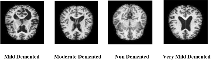
Medical applications have widely exploited machine learning (ML) techniques, which have shown considerable efficacy in determining the presence and diagnosis of numerous illnesses, including dementia, MCI, epilepsy, and Parkinson’s disease^13,14. As technology advances and the amount of data produced by brain-imaging methods increases, ML and deep learning (DL) become more critical for deriving pertinent and reliable information from brain-imaging data and accurately predicting AD. Especially, deep learning has transformed the pitch of medical imaging by allowing automated feature extraction, requiring less manual struggle, and giving more precise predictions¹⁵. Unlike traditional ML approaches, DL models can investigate massive and complex datasets, such as MRI and PET scans, to identify refined patterns and biomarkers related with AD^16,17. This ability is critical for early diagnosis and discriminating between stages of AD that would otherwise be extremely challenging for human experts to recognize. The classification of AD has been approached through various machine-learning techniques, and the models offer good performance¹⁸. Furthermore, some well-known deep learning architectures, such as auto-encoders, convolutional neural networks, deep belief nets, and multilayer perceptrons, have been used to classify AD and forecast the progression of MCI patients to AD¹⁹. Figure 1 shows the sample MRI scans of AD classes such as mild demented, moderate demented, non-demented, and very mild-demented.

Sample images of an Alzheimer’s Disease MRI dataset¹³.

Full size image

Fathi et al.²⁰ reviewed the importance of AD using deep learning techniques. They studied several recent works and discussed the importance of hyperparameters selection of deep learning models, selection of deep learning networks, and gaps in the recent studies. Zhen et al.²¹ presented another review article that discussed the importance of conventional ML and popular deep learning techniques for AD prediction. Ahmed et al.²² suggested a fully customized CNN architecture for classifying AD at the early stages. They used an ADNI MRI dataset of three classes and obtained an accuracy of 99%. Murugan et al.²³ demonstrated a DEMentia NETwork for AD prediction from the MRI images. The presented work was evaluated on the publically available dataset and obtained an accuracy of 95.23%. Mahendaran et al.²⁴ offered a deep recurrent neural network and embedded optimization for accurate AD prediction. They also performed some preprocessing to control the quality of the selected dataset. Tree-based and regression-based techniques are implemented to select features. Further, they consider the Bayesian Optimization for the performance improvement of the deep model. Zheng et al.²⁵ presented a graph neural network (GNN) with feature weights for AD prediction. The ADNI dataset was used for the evaluation, and improved accuracy was obtained. Ebrahimi et al.²⁶ presented a 3DCNN and transfer learning (TL) approach for AD prediction from MRI scans. The 3DCNN architecture is compared with pre-trained models that are trained through TL. The results show that the 3D CNN models increase the accuracy of an AD prediction by 96.88%. Nawaz et al.²⁷ presented an AD diagnosis system using deep features. They used deep features and classified using SVM, KNN, and RF. The model achieved 99.21% accuracy that was better than the existing techniques. Shankar et al.²⁸ introduced an CNN architecture for AD classification. The machine learning classifiers were employed for the features classification. On the trained model, 96.23% accuracy has been obtained.

In summary, the vision transformers and MobileNet architectures have shown some improved accuracy in recent years for the recognition of medical images such as skin cancer and brain tumors; however, these models are not utilized in a single framework. Using these models in a single framework can improve overall efficiency and accuracy due to multi-directional weights. This work considers the challenge of accurate AD prediction using a fused framework. In AD, the main challenge is similarity in classes such as Mild Demented and Moderate Demented. Also, these classes are similar to very mild demented classes. In addition, several studies used features of a single model for the classification, which can make it difficult to obtain better performance. In this work, we proposed a novel framework that consists of a new bottleneck self-attention model and a vision transformer. Features of both models are extracted and fused using a novel serially enhanced technique that is finally passed to shallow neural networks for classification. Our significant contributions to this work are as follows:

• A new customized deep learning model is designed based on inverted residual bottleneck blocks integrated with a self-attention mechanism (IRBwSA). The IRBwSA network contains residual parallel block in a reduction wise.

• Designed a vision transformer model according to the nature of the selected dataset and trained both models using fixed hyperparameters. The features are extracted from both models.

• Proposed a novel serially search-based technique for the fusion of extracted features of customized models.

• Best model is interpreted using an explainable AI technique named LIME for the insight information of an image.

This section presents a proposed AD prediction framework using deep learning and explainable AI using MRI scans. Figure 2 shows the proposed framework of AD prediction that illustrates the middle steps, such as data imbalance, model designing, training, features extraction and fusion, and classification. The dataset was acquired in the first step, and data augmentation techniques were executed. A novel inverted residual bottleneck model with self-attention has been designed, and training has been performed. Similarly, vision transformer architecture is employed to train on the augmented datasets. An explainable AI (LIME) technique diagnosed the disorder after the training phase and feature extraction. At the same time, features are obtained from a global average pool and self-attention layers and fused with the help of a novel approach. At the last stage, shallow neural network classifiers were applied for the final classification results. Each of the steps above is briefly described below.

Proposed framework of Alzheimer’s disease prediction.

Full size image

Dataset

An MRI dataset of AD²³ has been employed in this work for the experimental process available from an open-source platform, Kaggle (https://www.kaggle.com/datasets/tourist55/alzheimers-dataset-4-class-of-images). We have separated this dataset into four groups: mild demented, moderate demented, non-demented, and very mild demented. This dataset had 6400 images for training and testing purposes. Figure 3 illustrates images taken from each of the four categories. As shown in this figure, the number of images in each class is insufficient, and the dataset is imbalanced with 52 images and 2560 images.

Original dataset samples and summary of an Alzheimer Disease²³.

Full size image

Overfitting is a common issue in network training due to insufficient data, as the model struggles to forecast unseen occurrences due to network tuning. Inadequate sample size and uneven class distribution reduced the system’s efficacy, leading to less interpretable outcomes from minority samples²⁹. The deep learning models need a huge amount of data for learning; therefore, we performed dataset augmentation using flip and rotation techniques. The framework uses several augmentation elements, including rotating, zooming, shifting, shearing, and horizontal flipping³⁰. After applying the augmented technique, 12,800 images were found in the training and testing parts. Figure 4 illustrates the number of samples in each class.

Summary of the dataset after the augmentation process.

Full size image

Pre-trained vision transformer

The transformer architecture and the vision transformer architecture both include several degrees of self-attention. A network may discover long-term relationships in information without the need for repetition since each self-attention layer analyses the data that arrives in parallel.

The outcome based on the self-attention levels is processed further with a sequence of feed-forward layers that come after them. The vision transformer design is notable for its innovative use of multi-headed self-attention, which enables the network to concurrently attend to various aspects of the input data³¹.

An input to a typical transformer is a 1D sequence of token embeddings; hence, ViT reshapes the visual (Avarepsilon R^{M*N*O}) into a series of flattened 2D patches, ({text{A}}^{text{P}}upvarepsilon {text{R}}^{text{v}*({text{P}}^{2}*text{O})}), to deal with a 2D image, where (text{M}*text{N}) depicts the resolution of an original image. The symbol (text{O}) represents the number of channels, (P) displays the resolution of the image patch, and (text{b}=text{M}*text{N}/{text{P}}^{2}) represents the number of patches. Since vision transformers employ the same width for all layers, they flatten the patches and convert image patches to a dimensional vector (D) with a capable linear projection. The projection results represent the patch embedding.

Multi-Head Self Attention (MSA) and Multilayer Perceptron (MLP) are key components of the conventional transformer layers. The MSA divides the input into many parts and then measures each input’s scaled dot product in parallel. Following that, the slices of the attention outputs generate the final results of multi-head self-attention³². Mathematically, it is defined as follows:

At the top of the MSA layer, a multi-layered perceptron is applied. Layers of linearity in the MLP module were distinguished by applying a Gaussian Error Linear Unit (GeLU). Both MSA and MLP employ skip-connection-like residual networks and layer normalization. Mathematically, it is defined as follows:

where ({text{s}}_{text{t}-1}) shows for the (text{t}-1) layer, (LN) shows the linear normalization and ({s}_{t}) represents the output of the (text{t}) layer. Figure 5 shows the architecture of a vision transformer for AD prediction. In this work, we employed tiny16 ViT using the transfer learning concept. For achieving the transfer learning, The last three layers indexing, fully connected, and softmax are replaced with new GAP layer, new fully connected, and new softmax layer.

Architecture of a proposed vision transformer for AD prediction.

Full size image

Novelty: proposed IRBwSA architecture

In convolutional neural networks (CNN), the inverted residual bottleneck model is a popular design framework, especially in embedded and mobile device architectures. The MobileNetV2 architecture helped to popularize it. In a typical bottleneck block, the input feature map is first dimensionally reduced using a pointwise (1 × 1) convolution. The convolutional is then processed by a depth-wise separable convolution that expands back to its original dimensions using another pointwise convolution. The inverted residual bottleneck model reverses this structure. Instead of decreasing dimensionality, it expands it, performs a lightweight 3 × 3 depth-wise convolution, and finally returns to its required dimensions.

This paper proposes a new architecture based on residual blocks, parallel bottleneck structures, and self-attention mechanism. The employed multiple parallel block is inspired by the multi-branch architectures such as inception³³ which shows that parallel paths can enhance the representational power without increasing the computational complexity of the network. Figure 6 demonstrates the proposed architecture. The initial input dimensions in this network design are 227 × 227 × 3. The first convolutional layer and activation layer have a depth of 8, a filter size of 3 × 3, and a stride of 1. After that, a first inverted parallel residual block has been added.

Proposed architecture of an inverted-residual bottleneck model with self-attention.

Full size image

First parallel inverted residual bottleneck block

In the first stage, the six inverted residual bottleneck blocks are added in a parallel fashion, and each block consists of a ReLU activation³⁴ due to its stability and non-saturating nature, a batch normalization with 16 channels, a convolution layer with a depth of 16, a stride of 1, and a filter size of 1 × 1. A 3 × 3 filter-sized grouped convolution layer is added, followed by an activation layer, a batch normalization layer, and a convolution layer with a depth of 8, a filter size of 1 × 1, and a stride of 1. The remaining five blocks use the similar pattern to convolve the weights in the input layer. Finally, these blocks are joined together with an additional layer. Before adding the next parallel block, the network was updated with a few intermediate layers. A convolutional layer and activation layer with a depth of 8 are added, with a 3 × 3 filter size and stride of 2. The values of stride are employed strategically to perform down sampling while holding features richness.

Second parallel inverted residual bottleneck block

In the second step, five parallel inverted residual bottleneck blocks are introduced. The depth and other layers have the same settings as the First Parallel Inverted Residual Bottleneck Block (FPIRBB). Following this stage, a few intermediate layers were added, including a convolutional layer with a depth of 16, a filter size of 3 × 3, a stride value of 2, and a ReLu activation layer.

Third parallel inverted residual bottleneck block

The third level introduced a four-path parallel inverted residual bottleneck block. The current block consists of four pathways and one skip link, with a total of seven layers in each path. Each path begins with the convolution layer having filter size of 1 × 1, depth of 32, and stride of 1, followed by an activation layer (ReLU). Furthermore, batch normalization has been used to speed up the training process. After that, a grouped convolution layer with a filter size of 3 × 3 is added, followed by another activation layer, a batch normalization, and a convolution layer with a depth of 16 and a filter size of 1 × 1. All these weights (four paths) and skip connections have been added using an additional layer. A few intermediate layers, such as convolutional and ReLu activation, have been added, with a stride value of 2.

Fourth parallel inverted residual bottleneck block

The same procedure is followed in the fourth parallel inverted residual bottleneck block as in the third parallel block, with one exception: three pathways were added along with a skip connection. A depth size 32 was added to the intermediate layer with a stride of 2. Moreover, each convolutional layer is followed by a ReLU activation layer.

Fifth parallel inverted residual bottleneck block

In this stage, two paths are then appended in parallel, each including a convolution layer with a stride of 1, a depth of 64, and a filter size of 1 × 1, followed by a ReLU activation layer and a batch normalization layer with 64 channels. After that, a 3 × 3 filter-size grouped-convolution layer and a ReLU activation layer were added. In addition, a convolution layer with 32-depth, one stride, and 1 × 1 filter size was added at the end of this stage, and it was finally concatenated using an additional layer. After that, a few intermediate layers were added, similar to intermediate layer 4, with a stride value of 2.

Sixth and seventh parallel inverted residual bottleneck blocks

Single and dual paths are added in the sixth and seventh parallel residual blocks. There were two paths in the seventh block. In each path, two convolution layers are placed, the first having a stride of 1, number of filter is 128, a filter size of 1 × 1, and the second having a filter size of 1 × 1, 64, and a stride of 1. A grouped convolutional layer is also added of filter size 3 × 3. After both stages, a few intermediate layers of stride size 2 were added.

Additional blocks

In the next blocks, the convolutional layers are convolved on different depth sizes, such as 128 and 256. The filter size of each convolutional layer was 3 × 3 and a stride of 1. Before the final block, two paths were added. In each path, a convolution layer with a depth of 512, a 1 × 1 filter size, and a stride of 1 is placed, followed by the ReLU layer and batch-normalization layer having 512 channels. Next, a 3 × 3 grouped convolution is added to it. After that, a ReLU layer is inserted, and the next one is the batch-normalization layer. In the end, the convolution layer with a 1 × 1 filter dimension, a depth of 256, and a stride of 1 is applied.

Final layers

The model’s final addition layer connects these blocks to the other layers. After that, a convolution layer with a depth of 512, a stride of 1, and a 3 × 3 filter size has been added. Next, the global average pooling layer was added. Next, a flattening layer is added. It was used to reduce the multidimensional input to one dimension, which was typically used while transitioning from the convolution layer to the fully connected layer, followed by a fully connected layer 1 with 512 input-size in it, a self-attention layer, a new fully connected layer, a new Softmax layer, and an output layer for categorization. The cross entropy function is employed as a loss function of the proposed model which is mathematically formulated as: (mathop{intmkern-20.8mu circlearrowleft} {_{loss} } = – frac{1}{{phi_{s} }}mathop sum limits_{j = 1}^{{phi_{s} }} mathop sum limits_{k = 1}^{{Phi_{c} }} eta_{{j,Phi_{c} }} log left( {hat{eta }_{{j,Phi_{c} }} } right)), where ({Phi }_{c}) is the number of classes, ({phi }_{s}) is the number of samples, ({eta }_{j,{Phi }_{c}}) actual label for the sample ({j}^{th}) in class (k), and ({widehat{eta }}_{j,{Phi }_{c}}) is the predicated probability of the class (k) for sample (j). The total number of parameters of this proposed model is 3.4 million.

Hyperparameters and proposed models training

In this section, the hyperparameters of the proposed models are discussed. The selected dataset is divided into a 50:50 approach, and the training set is augmented. After that, the models are trained from scratch by employing several hyperparameters. The input size of each image for the presented models is (227times 227times 3). The frequency with which deep learning networks are trained using training and validation data is called epochs. In this work, we used 50 epochs for the training process. The next hyperparameter is the batch size. The batch size refers to the number of subsamples used concurrently in forwarding or backpropagation during network training. In this work, we selected the value of batch size of 64. The optimizer of this work is ADAM, and the learning rate is 0.00011. We use this learning rate due to the fast convergence rate. Moreover, the accuracy is utilized to validate the proposed model training performance.

After the setup of hyperparameters, both designed models are trained from scratch. The models are trained based on the number of epochs later utilized for feature extraction. In addition, features are extracted from the third last layers, such as self-attention and global average pool. The extracted features are finally fused using a novel serially controlled search update approach in the next step.

Novelty: proposed serially search-based fusion

Features are fused using a novel serially search-based approach. The proposed approach is based on two dependent steps. In the first step, features are fused using a serial approach and then passed to the search mechanism for the final fusion of the optimal features³⁵.

Consider, we have two feature vectors of dimensions (Ntimes 912) and (Ntimes 512). The feature vectors (left|O(v)right|) and (left|Q(v)right|) are mathematically represented as:

where, (left|O(v)right|) and (left|Q(v)right|) are feature vectors of the proposed vision and IRBwSA models. The serial fusion of these feature vectors is defined as follows:

where (left|Pright|) denotes the serially fused feature vector of dimension N × 1424. After that, we opted for a strategy like Eagle Search that moves in a spiral pattern to search for food in the selected feature space. Mathematically, the movement process in the search space is defined as follows:

where (R) denotes the number of search cycles in a feature space, and (theta) expresses the angles. In this paper, we used (theta) values of 45 and 270. The eagle is searching for the optimal solution (food) in the mentioned angles and selects the best points for the final fusion as follows:

The final fused vector is obtained on dimension N × 712 and is finally classified using shallow wide neural network and other neural network classifiers.

Shallow Wide Neural Network: the shallow wide network has various types based on different hidden layer and neuron in the hidden layers such as narrow neural networks (NNN), medium neural networks (MNN), wide neural networks (WNN), bi-layered neural networks (BNN), and tri-layered neural networks (TNN). The NNN has one input, hidden and output layer. The hidden layer contains 10 neurons and ReLU activation. The NNN are often less intricate, exhibiting lower computational expenses and less danger of overfitting. The MNN and WNN contains one input, hidden, output layers. The MNN has 25 neurons and WNN has 100 neurons with ReLU activation. The BNN has one input, two hidden layer, and one output layer. The each hidden layer is consist of 10 neurons and the activation is ReLU. These networks allows to learn the complex relationship among the input data. The TNN has one input, three hidden layers, and one output layer. Each hidden layer consist of 10 neurons and the network has ReLU activation. The TNN network has more expressive and complex than the other networks and it can learn hierarchical structures in the data. The final selected features are classified using a Shallow Wide Neural Network (SWNN) classifiers for the final classification.

Local interpretable model-agnostic explanations (LIME)

The fundamental concept of explainable AI (XAI) was expressed to declare the methodologies for developing machine learning frameworks for human dilettantes. XAI approaches are used to explain the model’s predictions, results, and flaws. With XAI, it is possible to characterize the model’s integrity, accuracy, and fairness. Local Interpretable Model-Agnostic Explanations (LIME) were used to estimate the selective competence of the machine learning model³⁶. The primary goal of LIME is to assess the essential features of the input data for the classification outcome. It will estimate the behavior of a deep learning model. Some steps are: (i) Segment the image into features; (ii) Generate synthetic image data by randomly including or excluding features. Each pixel in the exclude feature is regained with the average image pixel; (iii) Classify the synthetic image using the deep network; (iv) Fit a regression model; and (v) Calculate the importance of each feature using the regression models.

Experimental setup: This section presents the experimental findings of the suggested framework. Sect. “Alzheimer disease MRI dataset results” details the experimental procedure, which used an MRI dataset. The dataset was divided 50:50, and the testing set underwent ten-fold cross-validation. A variety of classifiers, such as tri-layered neural networks and shallow neural networks are used to provide the classification results. Several metrics, such as recall rate, precision rate, F1-Score, efficiency, time, and AUC, were utilized to evaluate each classifier’s performance. We have selected these metrics because it is correctly assess the model reliably and clinically apply to the condition. The TPR tells the models ability to correctly identify who has AZ disease this is critical, since we do not want to miss cases that are actually AZ. Precision examines how many predicted positive cases are true positive cases, limiting the risk of excessive false positive alarms leading to unnecessary complications and implementation. The F1-score shows a balance score when both false positive and false negative cases are important. The overall accuracy for predictions, could lead to misleading results in imbalanced datasets where the less cases of AZ. The False Negative Rate (FNR) states the proportion of cases classified as healthy cases when in fact they are AZ. AUC examines the case by individual threshold in the ability for the model to distinguish between healthy cases and diseases cases as well. Finally, time complexity in seconds reflects the model speed of predictions. The experiment was run on MATLAB 2023b on a desktop computer with 128 GB of RAM and a 12 GB NVIDIA RTX 3060 graphics card, using a deep learning toolkit.

Alzheimer disease MRI dataset results

In this section, the proposed framework is tested on an AD MRI dataset testing set using several experiments. In the first experiment, implemented vision transformer model features are extracted and classified. In the second experiment, the proposed inverted residual bottleneck model with self-attention is utilized and extracted features from the self-attention layer. The extracted features are classified using shallow neural networks and multi-layered neural networks. In the third experiment, the proposed fusion has been performed and classification results. The purpose of these experiments is to analyze the performance of each middle step during the classification phase.

Proposed vision transformer results

Table 1 displays the results of the vision transformer classification for the AD MRI dataset. The highest accuracy for the Shallow WNN (SWNN) classifier is shown in this table of 93.9%. The classifier’s estimated recall rate is 93.85%, the precision rate is 93.875%, FNR is 6.15, FPR is 0.02044, F1-Score is 93.68%, time is 3.8103 s, and AUC is 0.98, respectively. These values were calculated for the remaining classifiers as well, and it will appear from the numbers that SWNN performs better than the other classifiers. Figure 7A,B depict the confusion matrices that can be utilized further to verify the calculated recall and precision rates of SWNN. The computational time of each classifier is also noted during the classification method, and the MNN classifier has a lowest execution time of 2.731(sec). The TNN classifier consumed the highest execution time of 8.9804(sec).

Confusion matrix of SWNN after employing Vision Transformer. (A) Confirmation of recall rate (B) confirmation of precision rate.

Full size image

Proposed inverted residual bottleneck model with self-attention results

Table 2 shows the results for the inverted residual bottleneck model with self-attention classification. This table exhibits that the SWNN classifier achieved the highest accuracy of 85.6%. Other calculated performance measures such as TPR rate (85.625), PPV (85.675), F1-Score (85.649%), FNR (14.375), FPR (0.04791), time (3.4295 s), and AUC (0.961025), respectively. These measures are also computed for other classifiers in this table, and the SWNN outperforms are shown. Figure 8 illustrates the confusion matrix that can be used to further validate the SWNN performance in terms of recall rate and precision rate. In addition, each classifier’s computational time is also noted, and the Medium Neural Network classifier takes a minimum time of 2.6119 s. The Tri-layered neural network consumed a maximum time of 11.457 s. Comparing the results of this experiment with Table 2, it is noted that the proposed model performance is a little reduced than the vision model.

Confusion matrix of SWNN after employing inverted residual bottleneck with self-attention. (A) Confirmation of recall rate (B) confirmation of precision rate.

Full size image

Proposed fusion results

After the experimental process of individual feature extraction of both designed models, features are fused using a novel serially search technique. Results are presented in Table 3. In this table, the maximum obtained is an accuracy of 96.1% by the SWNN classifier. The improved PPV value of this classifier is 96.05%, a TPR value of 96.075%, and an F1-Score of 96.062%, respectively. Furthermore, Fig. 9 depicts the confusion matrix of the SWNN classifier. The computation times of each classifier are noted, and MNN is executed faster than the other classifiers. The shortest execution time for this classifier is 4.7267 s, while the longest is 16.758 s (sec) for the TNN classifier. Comparing the fusion results with Tables 2, 3, it is observed that the fusion of both proposed models significantly improved the accuracy and precision rates. Moreover, a minor increase occurred in the computational time after the fusion process that did not affect the overall performance of the proposed framework.

Confusion matrix of SWNN after employing the proposed fusion technique. (A) Confirmation of recall rate (B) confirmation of precision rate.

Full size image

Discussion

In the first ablation study, pre-trained models like inceptionv3, denseNet201, ResNet18, MobileNetv2 are compared with the proposed models based on the different splits of the dataset. The Fig. 10 shows the performance of each model on 50:50, 60:40, and 70:30 splits. The 50, 60, and 30 percent data is utilized for the training of models and 50, 40, and 30% data is employed for the testing process in different trials and it is observed the models are outperformed on 50:50 split. On this split, inceptionv3, denseNet201, ResNet18, MobileNetv2 achieved 95.1, 94.6, 91.8, 94.8% accuracy respectively and the proposed models achieved the highest accuracy of 96.1, and 98.9% of accuracy.

Proposed models evaluation on different splits of dataset.

Full size image

In second ablation study, we performed an eagle search mechanism with different variants to verify the method’s effectiveness. The fusion method is divided into three variants: serial fusion, eagle search without local exploitation, eagle search without global exploitation, and proposed eagle search fusion, as shown in Table 4. After dividing, each variant is performed, and the vector dimension and accuracy are measured. The serial fusion method achieved a 98.26% accuracy, and the vector dimension is quite high, which is (N times 1424), eagle search w/o global exploration achieved 92.49% accuracy with vector dimension (N times 596), and eagle search w/o local exploitation gained 89.67% accuracy and returned the dimension of N × 829. When we combine all the mechanisms in eagle search fusion, it achieves 99.54% accuracy with (N times 712) deminsion.

In the third ablation study, the pertained models and proposed models are evaluated using the static and dynamic hyperparameters as shown in Fig. 11. In this figure, it is presented that the inceptionv3, DenseNet201, MobileNetv2, ResNet18, and both proposed models (IRBWSA and ViT) are trained using the static hyperparameters which is described in Sect. “Hyperparameters and proposed models training” and grid search optimization method is implemented to dynamically selection of hyperparmeters including batch size, learning rate, optimizer, and epochs. The ranges of these hyperparameters are [16, 32, 64], [1 ({e}^{-6},{e}^{-2})], [ADAM, SGDM, RMSprop], and [20, 30, 50, 80], respectively. In this experiment, it is observed that the performance of models are quite improved by employing the grid search hyperparmeters method. The inception, densnet201, mobilenetv2, resnet18 accuracies are quite improved which is 0.5, 1.1, 0.1, and 0.3% respectively. However, the proposed models IRBwSA and ViT gained highest accuracies on static hyperparameters which are 96.1, and 98.9%. Therefore, the overall framework is evaluated using the static hyperparameters.

Proposed models evaluation using static and dynamic hyperpatameters tuning.

Full size image

In Table 5, ablation study is conducted among with deep learning models based on the parameters, model size, performance calculated using the Monte Carlo cross-validation method. According to the table, InceptionV3 has 23.9 M parameters and a small size of 23.9 MB, with a correspondingly excellent MCCV accuracy of 95.0% ± 1.2%. ResNet50 has 25.6 M parameters and a considerably larger size of 96 MB, correspondingly achieving a slight drop in accuracy of 92.1% ± 0.9%. MobileNetV2 was excellent in terms of efficiency by using 3.5 M parameters and 13 MB in size, unfortunately dropping in performance to 89.3% ± 1.7%. VGG19 achieved good accuracy of 90.7% ± 1.0% with a high number of 143.6 M parameters and a size of 535 MB. ViT-Large16 was resource-intensive with 307 M parameters and a model size of 924 MB and with accuracy of 93.4% ± 0.8%. However, the proposed ViT model showed the highest state-of-the-art accuracy of 98.9% ± 0.5% with considerably fewer parameters of 5.7 M and size of 22.6 MB and the proposed IRBwSA model is lightweight with only 1.3 M parameters and with 28.4 MB, while also showing considerable accuracy of 96.1% ± 0.7%. The proposed models are outperforming in terms of model size and number of parameters while achieving good accuracy.

Figure 12 illustrates the LIME and GradCam (explainable AI) visual results for the Alzheimer’s Disease MRI dataset using both proposed models. LIME is used to determine an image’s important elements for classification purposes. The data displayed in this figure are based on ten observations from a different class. After applying LIME and GradCam to an image, there are multiple colors, like brown, orange, and blue. These colors represent the strong and important points of an image. Moreover, these figures illustrate the actual and predicted labels. Based on the predicted labels, image important points are visualized. The visualization process shows that the proposed models are well-trained on the selected dataset.

LIME results using the MRI dataset for Alzheimer’s disease.

Full size image

Comparison with existing techniques

Table 6 shows a comparison of the proposed framework with the most recent approaches. In²³, MRI scans are used to create a framework for identifying Alzheimer’s disease using Convolutional Neural Networks (CNN). This approach produces high-resolution disease probability maps, allowing precise visualizations of individual risks and specific diagnoses. With an accuracy of 95.23%, a DEMentia Network (DEMNET) is proposed to identify the phases of dementia from MRI in³⁷, using Python code and deep learning to forecast and diagnose Alzheimer’s disease using vgg16 and 2D CNN, achieving 70.3% and 67.5% accuracy, respectively. In³⁸, the proposed automated method for early Alzheimer’s disease detection uses brain magnetic resonance imaging and transfer learning for multi-class classification, achieving 91.70% accuracy and surpassing previous methods, according to simulation findings. In³⁹, with an accuracy rate of over 95% for single and binary class classifications, automated pipelines and machine learning algorithms have proven useful in precisely detecting AD and its stages. In year 2024. Awaryi et al.⁴⁰, proposed an bilateral filtering method for preprocessing the AD images and train through a customized light weighted CNN. They achieved 93.45% accuracy and alatrany et al.⁴¹, presented explainable AI based machine learning method using the feature space reduction and SVM for the classification. They achieved 90.7% of accuracy. The proposed framework obtained the accuracy of 96.1% on the same dataset within 5.9846 s. Overall, the proposed framework performed better than the recent techniques.

Wilcoxon signed-rank test

The Wilcoxon signed-rank test is a nonparametric statistical technique for comparing two related samples. It is intended for situations in which the data does not adhere to a normal distribution or when the assumptions of parametric tests are disregarded. This study implements the Wilcoxon signed test analysis on classifiers to evaluate the significant difference among performances. Two classifiers have been selected based on the accuracy metrics such as SWNN and TNN (see Table 7). The SWNN classifier ({{varvec{tau}}}_{{varvec{H}}}) is selected based on the highest accuracy, and the TNN ({{varvec{tau}}}_{{varvec{L}}}) classifier is selected based on the lowest accuracy. Initially, the null and alternative hypothesis is assumed. ({Phi }_{h0}) denotes the null hypothesis, Φℎ0 assumes that there is a significant difference among the classifiers, and ({Phi }_{h1}) denotes the alternative hypothesis, ({Phi }_{h1}) assumes that there is no significant difference among the classifiers. After that, the difference between the performances is calculated using ({{varvec{C}}}_{{varvec{d}}{varvec{i}}{varvec{f}}{varvec{f}}}=({{varvec{tau}}}_{{varvec{H}}}-{{varvec{tau}}}_{{varvec{L}}})) and determined the absolute values of (|{{varvec{C}}}_{{varvec{d}}{varvec{i}}{varvec{f}}{varvec{f}}}|). Moreover, the absolute values are ranked from the smallest numbers ({{varvec{psi}}}_{{varvec{R}}{varvec{a}}{varvec{n}}{varvec{k}}{varvec{i}}{varvec{n}}{varvec{g}}}), as shown in Table 7. The sum of signed and unsigned ranks is calculated by using Eqs. (15 and 16).

where ({{varvec{psi}}}_{{{varvec{R}}}^{+}}) and ({{varvec{psi}}}_{{{varvec{R}}}^{-}}) presented the sum of positive and negative ranks, and the total value of ({{varvec{psi}}}_{{{varvec{R}}}^{+}}) is 6, while ({{varvec{psi}}}_{{{varvec{R}}}^{-}}) is 0 because there is no ({-}ve) rank values. The (n) denoted the number of selected samples in the test. After that, the mean and standard deviation are measured by using the Eqs. (17a and 17b).

where ({Phi }_{mu }) and ({Phi }_{sigma }) denoted the mean and standard deviation and the values are ({Phi }_{mu }=3) and ({Phi }_{sigma }=1.843). In the end, the value of ({z}_{score}) is measured using Eq. 18.

The value of ({z}_{score}=1.627). The significant level is set at 95%, which presents a value of 0.05. According to the ({z}_{table}) the critical value is 1.96. The ({z}_{score})>({z}_{table}). Thus, the null hypothesis ({Phi }_{h0}) is accepted, and it states that the performance among the classifiers has a significant difference.

Proposed architecture results on ADNI dataset

To further validate the proposed model, we also performed experiments using ADNI dataset^42,43. Patients with mild cognitive impairment (MCI), Alzheimer’s disease, and healthy controls are all included in the ADNI dataset. The ADNI includes clinical data, MRI and PET imaging, blood and CSF biomarkers, cognitive assessments, and genetic information⁴³. There are 1296 T1-weighted MRI scans in this dataset. With a resolution of 1.5 mm isotropic voxels, each scan creates a three-dimensional image of the brain. The scans are separated into five classes such as CN patients, EMCI, LMCI, AD, and MCI. More information of this dataset can be find in paper⁴². Table 8 presents the results of this dataset using proposed architecture and it is perceived that the fusion process achieved the highest accuracy of 99.8% for SWNN classifier. The recall rate is 99.88% that can be verified by a confusion matrix, illustrated in Fig. 13. Moreover, we also computed the results of Vision Transformer model and proposed Inverted Residual Bottleneck Model with Self-Attention architecture separately. The SWNN classifier gained 95.6% accuracy for Vision Transformer and 94.2% using IRB with self-attention. Hence, the proposed model also shows the better accuracy on ADNI dataset.

Confusion matrix of SWNN classifier after employing proposed fusion step.

Full size image

This work’s datasets are publicly available on the Mendaly platform and Kaggle. https://data.mendeley.com/datasets/ch87yswbz4/1 and https://www.kaggle.com/datasets/marcopinamonti/alzheimer-mri-4-classes-dataset. Also, the original reference for this dataset is given as: Yakkundi, Ananya (2023), “Alzheimer’s disease dataset”, Mendeley Data, V1,

1. Shakarami, A., Tarrah, H. & Mahdavi-Hormat, A. A CAD system for diagnosing Alzheimer’s disease using 2D slices and an improved AlexNet-SVM method. Optik 212, 164237 (2020).

   CAS  Google Scholar 

2. Khojaste-Sarakhsi, M., Haghighi, S. S., Ghomi, S. F. & Marchiori, E. Deep learning for Alzheimer’s disease diagnosis: A survey. Artif. Intell. Med. 130, 102332 (2022).

   CAS  PubMed  Google Scholar 

3. Guarino, A. et al. Executive functions in Alzheimer disease: A systematic review. Front. Aging Neurosci. 10, 437 (2019).

   PubMed  PubMed Central  Google Scholar 

4. Huang, S.-T., Loh, C.-H., Lin, C.-H., Hsiao, F.-Y. & Chen, L.-K. Trends in dementia incidence and mortality, and dynamic changes in comorbidity and healthcare utilization from 2004 to 2017: A Taiwan national cohort study. Arch. Gerontol. Geriatr. 121, 105330 (2024).

   PubMed  Google Scholar 

5. Brown, C. S. et al. Trends in cause-specific mortality among persons with Alzheimer’s disease in South Carolina: 2014 to 2019. Front. Aging Neurosci. 16, 1387082 (2024).

   PubMed  PubMed Central  Google Scholar 

6. Kouri, N. et al. Clinicopathologic heterogeneity and glial activation patterns in Alzheimer disease. JAMA Neurol. 81(6), 619–629 (2024).

   MathSciNet  PubMed  PubMed Central  Google Scholar 

7. Janghel, R. & Rathore, Y. Deep convolution neural network based system for early diagnosis of Alzheimer’s disease. Irbm 42(4), 258–267 (2021).

   Google Scholar 

8. Raghavaiah, P. & Varadarajan, S. A CAD system design for Alzheimer’s disease diagnosis using temporally consistent clustering and hybrid deep learning models. Biomed. Signal Process. Control 75, 103571 (2022).

   Google Scholar 

9. Lazli, L., Boukadoum, M. & Mohamed, O. A. A survey on computer-aided diagnosis of brain disorders through MRI based on machine learning and data mining methodologies with an emphasis on Alzheimer disease diagnosis and the contribution of the multimodal fusion. Appl. Sci. 10(5), 1894 (2020).

   CAS  Google Scholar 

10. Allioui, H., Sadgal, M. & Elfazziki, A. Utilization of a convolutional method for Alzheimer disease diagnosis. Mach. Vis. Appl. 31(4), 25 (2020).

    Google Scholar 

11. Raghavaiah, P. & Varadarajan, S. A CAD system design to diagnosize Alzheimers disease from MRI brain images using optimal deep neural network. Multimedia Tools Appl. 80(17), 26411–26428 (2021).

    Google Scholar 

12. Kumar, S. et al. Machine learning for modeling the progression of Alzheimer disease dementia using clinical data: a systematic literature review. JAMIA Open 4(3), ooab052 (2021).

    PubMed  PubMed Central  Google Scholar 

13. Mirzaei, G. & Adeli, H. Machine learning techniques for diagnosis of alzheimer disease, mild cognitive disorder, and other types of dementia. Biomed. Signal Process. Control 72, 103293 (2022).

    Google Scholar 

14. Park, J. H. et al. Machine learning prediction of incidence of Alzheimer’s disease using large-scale administrative health data. NPJ Dig. Med. 3(1), 46 (2020).

    Google Scholar 

15. Lilhore, U. K. et al. Optimizing protein sequence classification: integrating deep learning models with Bayesian optimization for enhanced biological analysis. BMC Med. Inform. Decis. Mak. 24(1), 236 (2024).

    PubMed  PubMed Central  Google Scholar 

16. Mazhar, T. et al. A novel expert system for the diagnosis and treatment of heart disease. Electronics 11(23), 3989 (2022).

    CAS  Google Scholar 

17. Lilhore, U. K. et al. An attention-driven hybrid deep neural network for enhanced heart disease classification. Expert. Syst. 42(2), e13791. https://doi.org/10.1111/exsy.13791 (2025).

    Article  Google Scholar 

18. AlSaeed, D. & Omar, S. F. Brain MRI analysis for Alzheimer’s disease diagnosis using CNN-based feature extraction and machine learning. Sensors 22(8), 2911 (2022).

    ADS  PubMed  PubMed Central  Google Scholar 

19. Abrol, A. et al. Deep residual learning for neuroimaging: an application to predict progression to Alzheimer’s disease. J. Neurosci. Methods 339, 108701 (2020).

    PubMed  PubMed Central  Google Scholar 

20. Fathi, S., Ahmadi, M. & Dehnad, A. Early diagnosis of Alzheimer’s disease based on deep learning: A systematic review. Comput. Biol. Med. 146, 105634 (2022).

    PubMed  Google Scholar 

21. Zhao, Z. et al. Conventional machine learning and deep learning in Alzheimer’s disease diagnosis using neuroimaging: A review. Front. Comput. Neurosci. 17, 1038636 (2023).

    PubMed  PubMed Central  Google Scholar 

22. A. W. Salehi, P. Baglat, B. B. Sharma, G. Gupta, and A. Upadhya, A CNN model: earlier diagnosis and classification of Alzheimer disease using MRI. In 2020 International Conference on Smart Electronics and Communication (ICOSEC), 156–161. (2020).

23. Murugan, S. et al. DEMNET: a deep learning model for early diagnosis of Alzheimer diseases and dementia from MR images. IEEE Access 9, 90319–90329 (2021).

    Google Scholar 

24. Mahendran, N. A deep learning framework with an embedded-based feature selection approach for the early detection of the Alzheimer’s disease. Comput. Biol. Med. 141, 105056 (2022).

    PubMed  Google Scholar 

25. Zeng, L., Li, H., Xiao, T., Shen, F. & Zhong, Z. Graph convolutional network with sample and feature weights for Alzheimer’s disease diagnosis. Inf. Process. Manage. 59(4), 102952 (2022).

    Google Scholar 

26. A. Ebrahimi, S. Luo, and R. Chiong, Introducing transfer learning to 3D ResNet-18 for Alzheimer’s disease detection on MRI images. In 2020 35th international conference on image and vision computing New Zealand (IVCNZ), 1–6. (IEEE, 2020).

27. Nawaz, H. et al. A deep feature-based real-time system for Alzheimer disease stage detection. Multimedia Tools Appl. 80, 35789–35807 (2021).

    Google Scholar 

28. Shankar, K. et al. Alzheimer detection using Group Grey Wolf Optimization based features with convolutional classifier. Comput. Electr. Eng. 77, 230–243 (2019).

    Google Scholar 

29. Afzal, S. et al. A data augmentation-based framework to handle class imbalance problem for Alzheimer’s stage detection. IEEE Access 7, 115528–115539 (2019).

    Google Scholar 

30. AbdulAzeem, Y., Bahgat, W. M. & Badawy, M. A CNN based framework for classification of Alzheimer’s disease. Neural Comput. Appl. 33(16), 10415–10428 (2021).

    Google Scholar 

31. Odusami, M., Maskeliūnas, R. & Damaševičius, R. Pixel-level fusion approach with vision transformer for early detection of Alzheimer’s disease. Electronics 12(5), 1218 (2023).

    Google Scholar 

32. Hoang, G. M., Kim, U.-H. & Kim, J. G. Vision transformers for the prediction of mild cognitive impairment to Alzheimer’s disease progression using mid-sagittal sMRI. Front. Aging Neurosci. 15, 1102869 (2023).

    PubMed  PubMed Central  Google Scholar 

33. C. Szegedy et al., Going deeper with convolutions. In Proceedings of the IEEE conference on computer vision and pattern recognition. 1–9. (2015).

34. A. F. Agarap, Deep learning using rectified linear units (relu). https://arXiv.org/abs/1803.08375. (2018).

35. Khan, M. A. et al. Optimal feature selection for heart disease prediction using modified Artificial Bee colony (M-ABC) and K-nearest neighbors (KNN). Sci. Rep. 14(1), 26241 (2024).

    CAS  PubMed  PubMed Central  Google Scholar 

36. Sekaran, K. & Alsamman, A. M. Bioinformatics investigation on blood-based gene expressions of Alzheimer’s disease revealed ORAI2 gene biomarker susceptibility: An explainable artificial intelligence-based approach. Metab. Brain Dis. 38(4), 1297–1310 (2023).

    CAS  PubMed  PubMed Central  Google Scholar 

37. Mggdadi, E., Al-Aiad, A., Al-Ayyad, M. S. & Darabseh, A. Prediction Alzheimer’s disease from MRI images using deep learning. In 2021 12th International Conference on Information and Communication Systems (ICICS) 120–125 (IEEE, 2021).

    Google Scholar 

38. Ghazal, T. M. et al. Alzheimer disease detection empowered with transfer learning. Comput. Mater. Continua 70(3), 5005–5019 (2022).

    Google Scholar 

39. Shukla, A., Tiwari, R. & Tiwari, S. Review on Alzheimer disease detection methods: Automatic pipelines and machine learning techniques. Science 5(1), 13 (2023).

    Google Scholar 

40. Awarayi, N. S., Twum, F., Hayfron-Acquah, J. B. & Owusu-Agyemang, K. A bilateral filtering-based image enhancement for Alzheimer disease classification using CNN. PLoS ONE 19(4), e0302358 (2024).

    CAS  PubMed  PubMed Central  Google Scholar 

41. Alatrany, A. S., Khan, W., Hussain, A., Kolivand, H. & Al-Jumeily, D. An explainable machine learning approach for Alzheimer’s disease classification. Sci. Rep. 14(1), 2637 (2024).

    ADS  CAS  PubMed  PubMed Central  Google Scholar 

42. El-Assy, A., Amer, H. M., Ibrahim, H. & Mohamed, M. A novel CNN architecture for accurate early detection and classification of Alzheimer’s disease using MRI data. Sci. Rep. 14(1), 3463 (2024).

    ADS  CAS  PubMed  PubMed Central  Google Scholar 

43. ADNI, The Alzheimer’s disease neuroimaging initiative (ADNI). https://adni.loni.usc.edu/, (2023).

Download references

Authors and Affiliations

1. Department of Computer Science, HITEC University, Taxila, Pakistan

   Wardah Ibrar & Ameer Hamza

2. Department of Artificial Intelligence, Prince Mohammad Bin Fahd University, Al-Khobar, KSA, Saudi Arabia

   Muhammad Attique Khan

3. Department of Computer Engineering, College of Computing and Informatics, University of Sharjah, 27272, Sharjah, United Arab Emirates

   Saddaf Rubab

4. College of Computer Science, King Khalid University, Abha, Saudi Arabia

   Omar Alqahtani & M. Turki-Hadj Alouane

5. Department of ICT Convergence, Soonchunhyang University, Asan, 31538, Korea

   Sokea Teng & Yunyoung Nam

Contributions

All authors contributed equally in this manuscript.

Corresponding authors

Correspondence to Muhammad Attique Khan or Yunyoung Nam.

Competing interests

The authors declare no competing interests.

Publisher’s note

Springer Nature remains neutral with regard to jurisdictional claims in published maps and institutional affiliations.

Open Access This article is licensed under a Creative Commons Attribution-NonCommercial-NoDerivatives 4.0 International License, which permits any non-commercial use, sharing, distribution and reproduction in any medium or format, as long as you give appropriate credit to the original author(s) and the source, provide a link to the Creative Commons licence, and indicate if you modified the licensed material. You do not have permission under this licence to share adapted material derived from this article or parts of it. The images or other third party material in this article are included in the article’s Creative Commons licence, unless indicated otherwise in a credit line to the material. If material is not included in the article’s Creative Commons licence and your intended use is not permitted by statutory regulation or exceeds the permitted use, you will need to obtain permission directly from the copyright holder. To view a copy of this licence, visit http://creativecommons.org/licenses/by-nc-nd/4.0/.

Reprints and permissions