Artificial intelligence based classification and prediction of medical imaging using a novel … – Nature

The modern healthcare system uses several medical imaging modalities, including radiography, endoscopy, nuclear medicine imaging, CT scanning, mammography, ultrasound, MRI (magnetic resonance imaging), and pathology diagnosis¹. The analysis of medical images might be more complicated and longer due to the unavailability of radiologists (less experienced radiologists). Numerous clinical applications, such as early disease detection, diagnosis, treatment evaluation, and disease development tracking, depend heavily on medical imaging². A precondition for understanding computer vision-related medical image analysis is knowledge about deep learning techniques and artificial neural networks³. The field of study in medical image processing that is becoming more popular every day is deep learning (DL)⁴. DL is used extensively in medical imaging to determine the presence or absence of disease and classify the disease stage and type⁵.

In skin cancer, melanoma has emerged as the deadliest form of cancer over the past three decades, primarily due to its incidence rising. Melanocyte cells are the point of origin for the malignant lesion, typically called melanoma, which ultimately metastasizes through the epidermis. Data from the World Health Organization (WHO) show that in only one year, 2019, 11,650 Americans lost their lives to skin cancer⁶. The second common cancer, especially among women, is breast cancer, which begins in spreads to other parts of the body from the breast areas⁷. Breast cancer is the second most frequent disease in the world, affecting the breast tissue. The World Health Organization (WHO) reported that 6.6% of patients died from breast cancer, and 8.4% of patients were diagnosed⁸. Another crucial cancer name is lung cancer⁹.

On the other hand, early detection significantly raises the lung cancer survival rate. Pulmonary nodules are tiny cell growths that can be benign or cancerous inside the lung. Global Cancer Statistics reports that in 2018, lung cancer accounted for 1,761,007 (18.4% of all sites) fatalities and 2,093,876 (11.6% of all sites) new cases¹⁰. Gastrointestinal tract (GIT) infection and Oral cancer have also spread cancer types in the last decade¹¹. The most common GIT infections are esophagitis, bleeding, ulcers, and polyps. According to the American Cancer Society (ACS), older people are the main population affected by stomach illnesses. Twenty-seven thousand six hundred people in the US get stomach cancer, and 11,010 of them die from the disease^12,13.

Image technologies include various tools and methods for creating, adjusting, and interpreting digital visual output¹⁴. In the healthcare sector, medical imaging technologies like MRIs and X-rays aid in diagnosis, while facial recognition technology uses image analysis for security and identification¹⁵. Several other medical image technologies include Dermoscopy, Ultrasound, Chest X-ray, and WCE/CE. Computer-aided diagnosis (CAD) technology attempts to obtain a quantitative opinion to improve the clinical diagnostic procedure¹⁶. Among CADs, the primary objective is the ability to discriminate between benign and malignant tumors and lesions automatically. In many CAD instances, the choice and application of calculated features are equally crucial¹⁶.

Feature extraction is a necessary process that is often the first step in both data analysis and machine learning (ML). It identifies the most salient information in a raw data set to extract features that carry relevant information about noteworthy patterns or attributes¹⁷. To this end, the data that has been reduced in real-time and could be of high dimensionality is then reduced in size to a feature that encodes only the most essential pattern, attribute, or signal. Feature extraction seeks to improve algorithm performance by feeding machine learning algorithms^18,19.

A crucial step in ML is feature selection, where characteristics that significantly improve a model’s forecasting ability are kept and others eliminated from the dataset²⁰. Some benefits of feature selection include improved interpretability, lower risk of over-fitting, and better model performance, which makes it easier to gain meaningful insights from the model²¹. The best way to select features will vary based on the objectives of the investigation or the type of data, such as determining the most suitable approach for a given ML problem, which may entail trying several approaches. A branch of machine learning (ML) called “deep learning” (DL) utilizes multi-layered neural networks, or “deep neural networks” (DNN), to learn hierarchical representations of the data²² automatically. DL models eliminate the need for human feature engineering by automatically identifying and extracting complex patterns and features from raw data, in contrast to traditional ML techniques²³. The development of deep learning can be attributed to advancements in technology, such as GPUs, large datasets, and powerful computing resources²⁴. The key challenges of this work are as follows: i) An imbalanced dataset is a critical challenge that impacts the training of a model (increases the probability of a class that has a higher number of images) and later reduces the classification accuracy; ii) higher number of training parameters of a network not only increases the complexity but also remove the essential features in the training phase; iii) extraction of features from the raw images may contain some redundant and irrelevant information; therefore, it is a chance of misclassification. To resolve these challenges, We suggested a novel deep learning-based architecture that decreased computation time and increased classification accuracy. The following are our main contributions to this work:

• To overcome the problem of imbalancing, a data augmentation technique is performed on the selected datasets. In this step, the flip and rotate operations are performed.

• A novel self-attention-based convolutional neural network (CNN) architecture has been designed based on several weight layers and a self-attention module.

• A new lightweight inverted residual with multiscale weight layers architecture is designed to empower the learning process of the selected datasets.

• Features are extracted from the trained models and fused using a modified serial fusion with a strong correlation. The fused vector is optimized with an optimization algorithm—slap swarm controlled standard Error mean (SScSEM). The selected features are finally classified using neural networks.

• Detailed ablation studies were performed to verify the proposed model’s effectiveness. In addition, an explainable AI technique has been applied to interpret designed CNN models.

Medical imaging has shown significant success in the last decade using deep learning techniques for diagnosing and classifying diseases. Several computer vision techniques are presented for imaging modalities such as dermoscopy, ultrasound, and mammography²⁵. The researchers focused on contrast enhancement, segmentation, feature extraction, reduction of irrelevant features, and classification²⁶. Neslihan et al.²⁷ presented a breast cancer treatment technique based on deep learning. In the presented approach, they predicted the degree of image malignancy and the probability of malignant tumors using a CNN-based model. They achieved an accuracy of 82.13% on the selected dataset. The limitation of the presented approach was the task-wise early pausing in the multitasking. Zebari et al.²⁸ presented a DL approach for breast cancer classification. They used the ML to extract the region of interest (ROI). The ROI is further split into various blocks and extracted features that are later optimized through a genetic algorithm (GA). The presented approach obtained an improved accuracy of above 90%. The limitation of this technique was that many features were extracted from each block. There is another DL technique presented by Wu et al.²⁹ for breast cancer classification. They presented a DL approach for classifying breast cancer. They also employed ML algorithms such as support vector machine (SVM). They compared the performance with DL, in another work presented by Huynh et al.³⁰ for the breast cancer classification using transfer learning of the pre-trained CNN models. They extracted deep features from the dense layer and performed classification through SVM. An improved accuracy rate of 90% was obtained by this approach on the selected datasets. In another work presented by Mambou et al.³¹ for the breast cancer classification using DL. They employed a path-based CNN model and obtained 92% accuracy.

Several studies have recently been introduced to classify skin cancer from dermoscopy images³². Razzia et al.³³ presented a lightweight S-MobileNet architecture for classifying skin cancer from dermoscopic images. The Gaussian and SFTA techniques were initially used for preprocessing and segmentation. Later on, the resultant output is passed on to S-Mobilenet for final classification. The HAM10000 dataset was used for the experiment, and increased accuracy resulted. Hosney et al.³⁴ presented a deeply explainable inherent architecture for classifying multiclass skin lesions. The explainable technique was employed to interpret the local and global values of the network. In addition, the physician provides visual information in this architecture. The HAM10000 dataset was used for the experiment, and noteworthy results were achieved. Jinnai et al.³⁵ presented a framework for the skin cancer classification using DL. In the presented framework, they utilized FRCNN architecture and evaluated the performance on dermoscopic images. As a result, they achieved 86% accuracy. The limitation of the presented framework was the incorrect information extraction of the lesion area that, in turn, impacted the training of a neural network. Dildar et al.³⁶ presented a classification approach to skin cancer using DL. They selected the best deep learning model based on accuracy after initially evaluating the performance of other models. Fraiwan et al.³⁷ presented a deep transfer learning approach for the classification of skin cancer. They used thirteen pre-trained models and performed feature extraction and training using TL.

Jang et al.³⁸ presented a deep learning-based method for gastric cancer subclassification. Using a CNN-based algorithm, they achieved a 93% prediction accuracy for stomach tumors. The main limitation of this work was black because the DL models limit their interpretability and remain a significant barrier to their validation and clinical use. Ayyaz et al.³⁹ presented a classification scheme to detect endoscopic lesions for endoscopy videos. They employed a hybrid deep learning model based on CNN and obtained an accuracy above 90%. Mark et al.⁴⁰ presented a method for classifying lung cancer using deep learning. In the presented work, they employed pre-trained models such as VGG16 and inceptionV3. In the final stage, they obtained a classification output of 95%. Wang et al.⁴¹ presented a deep-learning approach for the early diagnosis and classification of lung cancer. Fati et al.⁴² presented a deep CNN architecture for classifying oral squamous cell carcinoma. The CNN models (Alex-Net and ResNet-18) used in this framework and integrated their information using local binary pattern (LBP), discrete wavelet transform (DWT), fuzzy color histogram (FCH), and grey-level co-occurrence matrix (GLCM). They obtained an improved accuracy of 99% on the selected dataset. A few more studies focused on lung cancer^43,44 and oral cancer^45,46.

The studies mentioned above focused on the pre-trained models, preprocessing, segmentation of cancer regions, and feature selection. In the preprocessing phase, noise is usually removed through some filtering techniques. Segmentation is the process that extracts the important regions; however, in deep learning, the incorrect regions mislead classification accuracy. In addition, the extracted features contain a few redundant information; therefore, designing a model that extracts only necessary information is essential. However, a feature selection technique must be modified or chosen based on the redundant information in a few cases. Considering such gaps, we proposed a new framework for classifying medical imaging using deep learning and explainable AI (XAI).

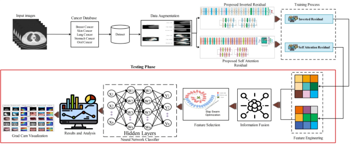
A new framework is proposed in this work for the classification and diagnosis of medical diseases using multi-type imaging techniques. The proposed framework is shown in Fig. 1. This figure shows that the data augmentation is performed at the first stage on all selected datasets of different cancers such as breast, skin, lung, stomach, and oral cancer. After that, two novel custom deep learning architectures, inverted residual and self-attention, were introduced. Both models are trained on the augmented datasets with manual hyperparameter selection. After the training process, features are extracted using the testing images of each dataset. The extracted features are fused using a modified serial fusion with a strong correlation. Further, the fused vector is optimized with an optimization algorithm- slap swarm controlled standard Error mean (SScSEM). For the final classification, neural network classifiers are used to classify the chosen features. GradCAM, an explainable artificial intelligence (XAI) approach, is used to analyze custom models. The detailed description of each step in this figure is discussed in the subsections below.

Proposed framework for the classification and diagnosis of medical diseases.

Full size image

Dataset collection

This work selects five cancer types for the classification: skin cancer, breast cancer, lung cancer, oral cancer, and stomach. For skin cancer, the ISIC2018 dataset has been selected. Similarly for the rest of the cancers, IN-breast, Lung cancer Imaging (https://www.kaggle.com/datasets/adityamahimkar/iqothnccd-lung-cancer-dataset), Oral cancer imaging (https://www.kaggle.com/datasets/smahmedhassan/oral-cancer-dataset), and Kvasir (https://www.kaggle.com/datasets/meetnagadia/kvasir-dataset) are selected. In the INbreast dataset, there are two classes: benign and malignant. There are eight classes in the Kvasir dataset: ulcerative colitis, polyps, normal-cecum, normal-pylorus, normal-z-line, dyed-lifted-polyps, and dyed-resection-margins. The lung cancer dataset contains three classes: benign, malignant, and normal. The Oral cancer imaging dataset has two classes: cancer and non-cancer. The ISIC2018 dataset includes seven classes: AK, BCC, BKL, DF, MEL, NV, and VASC. A few sample images of selected datasets are shown in Fig. 2. Moreover, Table 1 contains the summary of selected datasets.

Sample images of the selected datasets.

Full size image

Dataset augmentation

Data augmentation is a process in deep learning that increases the number of images or data to improve the learning process of a network⁴⁷. This work employs five datasets to train and validate the proposed framework⁴⁸. We split these datasets into Training (50%) and Testing (50%). As mentioned in Table 1, the number of images in each dataset is insufficient; therefore, increasing them using a few traditional geometric operations is essential. These operations not only increase the data but also enhance the diversity of the dataset. Three operations are rotation 90°, flipping horizontally, and vertically, as shown in Fig. 3. In the augmentation process, we considered a minimum of 4000 for the INbreast dataset, 32,000 for Kvasir, 6000 for Lung cancer, 4000 for Oral cancer, and 35,000 for ISIC-2018. A detailed overview of the augmented data is shown in Table 1. Mathematically, it is formulated as follows:

Visual description of data augmentation phase.

Full size image

Consider the input image of dimension (s times b) can be represented using the notation (left(T(x,y)right),) where (x) represents the row pixels (left{xin left(text{1,2},3dots ..,sright)right}) and (y) identifies the column pixel values (left{yin left(text{1,2},3dots ..,cright)right},) whereas the number of channels is three. The flip right, flip left, and rotation 90 are defined as follows:

where ({t}_{left(x, yright)}^{Left}) indicates flip left, ({T}_{left(x,yright)}^{Right}) denotes flip right, and by flipping right indicates ({T}_{left(x,yright)}^{Right}), and Rotate 90 degrees is indicated by ({t}_{left(x,yright) }^{Rot90}) . Figure 3 represents the visual description of these operations.

Proposed deep architectures

In this section, we presented the proposed deep architecture designed from scratch for medical imaging classification.Below is aA detailed description of the designed modelw.

Proposed 94-layered deep inverted residual architecture

This work proposes A new architecture named 94-layered Deep inverted for medical imaging classification. The proposed architecture is based on the concepts of residual blocks in an inverted fashion⁴⁹. The purpose of inverted residual blocks is to decrease the number of channels compared to the typical residual blocks. Usually, the residual blocks increase the number of channels at the beginning of the block⁵⁰. However, the lightweight inverted residual model is required to classify multiple objects efficiently, especially for medical diseases. The proposed lightweight model extracts deeper information about an image and reduces computing costs⁵¹.

The proposed architecture consists of five parallel and two serial-based blocks with an input size of (224times 224times 3). The initial convolutional layer has a stride value of 2, a kernel size of 3 × 3, and a depth size of 16. A ReLU activation layer has been added after this layer that follows the first parallel block. The first parallel block contains a grouped convolutional layer with a kernel size of (3times 3), a depth size of (16), and a stride value of 1. The convolutional in this block contains a depth size of 16 with a kernel size of (3times 3) and stride 1. After this weight layer, two layers, batch normalization, and RELU activation, were added. The second inverted parallel residual block included a grouped convolutional, ReLU activation, convolutional, and batch normalization layer. The grouped convolutional layer contains a depth size of 32, a kernel size of (3times 3), and a stride value of 1. The batch normalization and RELU activation layers have been added after this layer that is further connected with a convolutional layer of depth size (32), kernel size of (3times 3), and stride value of 1. The remaining two parallel inverted blocks contain grouped convolutional and convolutional layers of depth size 64 and 128, respectively. Also, the kernel size of (3times 3) and stride value of 1 is opted.

The series inverted residual block consists of grouped convolution and convolutional layers. Grouped convolutional layers have 256 depths and 3 × 3 kernels with stride values 1. The second convolution of this block contains a depth size of (256) and is connected with Layers for batch normalization and ReLU activation. The remaining two series blocks also contain a grouped convolution layer, convolutional layer, and ReLu activation layer. The depth size of the grouped CONV layer is (512), kernel size (3times 3), and a stride value of 1. The convolutional layer’s depth value is 1024, and side 1 has a similar kernel size. Three convolution layers with batch normalization are connected after the seventh inverted block. The RELU activation and grouped convolution layers have been included with a depth size of (1024), kernel size of (3times 3), and a stride value of 2 and 1, respectively. Finally, the global average pool layer, which is connected to the fully connected layer, and the Softmax layer have been added. The designed model contains 5.3 million total parameters and 94 layers. From 94 layers, there are 26 weight layers (convolutional). Figure 4 shows the architecture of the designed inverted residual-based CNN.

Proposed inverted residual architecture.

Full size image

Proposed 84-layered self-attention architecture

In recent neural network architectures, the self-attention residual block plays a vital role, especially in computer vision and natural language processing tasks, where the ability to capture long-range relationships is essential⁵². This block integrates residual connections and self-attention processes to enable information flow between various input data segments⁵³. The proposed 84-layered self-attention architecture consists of a total of 84 layers. In this architecture, we added seven self-attention residual blocks. In addition, each block consists of four parallel residual blocks and three series layers of residual blocks.

The proposed self-attention architecture takes an input size of (224times 224times 3). After the input layer, a convolutional layer of depth size 16, kernel size (3 times 3), and stride two has been added. A RELU activation layer follows the convolutional layer. After that, the first parallel residual block was added. The first parallel block consists of one batch normalization layer, two RELU activations, and one convolution layer with a kernel size of (3 times 3 ,) depth size of (16), and stride value of 1. The batch normalization layer comes after the RELU activation layer in the second block. This layer is connected to two other RELUs and one convolution layer with (3 times 3) kernel size, (32) depth size, and stride value of 1. The remaining two parallel blocks contain a convolution layer of depth size (64) and (128), with a kernel size of (3 times 3) and stride value of 1.

The fifth book, a series residual block, consists of three RELU activation layers, batch normalization, and convolutional layers. The convolution layer contains 128 depth size, (3times 3) kernel size, and stride 1. The remaining two series residual blocks also contain the same layer pattern; however, the depth size of the convolution layer is increased to 512 and (1024), respectively. After the series blocks, three convolutional layers of depth size 1024, filter size 3 × 3, and stride two have been added. A global average pooling layer is added, followed by a flattened layer. A self-attention layer has been added after the flattening layer. In the self-attention layer, features are transformed in the softmax function that returns a self-attention map. Lastly, the model has been trained for additional testing by adding fully linked softmax and classification layers. The proposed architecture consists of 7.5 million parameters and 17 convolutional layers. The architecture of the proposed 84-layered self-attention residual CNN is depicted in Fig. 5.

Proposed self-attention residual block architecture for medical imaging classification.

Full size image

Proposed networks training

The training process for the proposed architectures is discussed in this section. In the training process, selected datasets are divided into training and testing sets (50:50). Afterward, hyperparameters are initialized using salp swarm optimization, as mentioned in Section “Proposed feature optimization salp swarm algorithm (SSA)”. The initialized hyperparameters are an initial learning rate of 0.00021, momentum value of 0.701, batch size of 64, and ADAM as an optimizer. In addition, 50 epochs were performed to train a model. After the training process, the features are extracted in the testing phase. In the training phase, the proposed models obtained accuracy above 90%.

Proposed framework testing phase

In this section, we discuss the testing phase of our proposed work based on the trained models of several types of medical imaging. In the testing phase, features are first extracted from the trained model. Figure 6 illustrates the workflow of the testing phase. This figure describes that the testing images are acquired for the selected five different datasets and passed to trained models for feature extraction. The Global Average Pool (GAP) and Self-Attention layers extract features. In that order, the retrieved feature vector’s dimensions are N × 1024 and N × 1024. The retrieved features are merged in the following stage using a novel serial-based strong correlation technique. After that, the fused features are optimized using a slap swarm-controlled standard error mean (SScSEM) optimization algorithm. The final features are fed into shallow neural network classifiers for the final classification. In addition, the GRAD-CAM technique is employed to interpret the design models.

Proposed testing process for the medical image classification.

Full size image

Serial strong correlation fusion

Fusion is the amalgamation of data from two or more sources to increase the framework’s effectiveness. We proposed a fusion technique called serial-based strong correlation in this work. In this approach, features are initially fused using a serial approach⁵⁴ that is mathematically expressed as follows:

Consider the following two feature vectors: (alpha) and (ss) having dimensions (Mtimes {N}_{1}) and (Mtimes {N}_{2}). Where (M) represents the number of testing samples and ({N}_{1}, {N}_{2}) denotes the extracted features. The Pearson Correlation Coefficient is computed using the following equation:

where (left(rU and Vright)) denote the Pearson Correlation, (overline{U }) and (overline{V }) are sample means of (U) and (V) features, respectively. The (rleft(U,Vright)) can be further computed by the following equation:

The (rleft(alpha ,beta right)) return a value in between [-1,1]. However, in our case, we consider (rleft(alpha ,beta right)>1), which means a positive correlation among features. This entire process was continued, and finally, strong correlated features are combined using a serial approach.

where ({S}_{(v)}^{fuse}) denotes the final fused vector, the resulting vectors are (Ntimes 1282), (Ntimes 1426), (Ntimes 1202), (Ntimes 1510), and (Ntimes 1308), respectively, for breast cancer, skin cancer lung cancer, stomach cancer, and oral cancer, respectively. The fused vector is further optimized using slap swarm controlled standard Error mean (SScSEM) optimization that, in return, selects the best features for the improved classification.

Proposed feature optimization salp swarm algorithm (SSA)

A recent optimization technique created to handle different kinds of optimization problems is the Salp Swarm Algorithm (SSA)⁵⁵. Salps are a type of planktonic tunicate that belongs to the Salpidae family. Their behavior is similar to that of salps in the wild⁵⁶. Furthermore, their tissues and movement patterns bear similarities to jellyfish, as does the high water content in their weights⁵⁷. They move by contracting; thus, their locations are altered when water is pumped through their jelly bodies. Through quick, harmonic shifts, salps in the sea display a swarm behavior called the salp chain, which may help with better feeding and movement⁵⁸. Based on this behavior, the authors created a mathematical model of salp chains and evaluated it in optimization tasks.

The first step adopted by SSA is to split the population into two groups: followers and leaders. The salps in the chain are referred to as followers and leaders, respectively⁵⁹. The salps position is calculated in n-dimensions, where n is the number of variables in the search space. These salps seek out a food supply, indicating the swarm’s intended aim. Since it is recommended that the position be updated by using the following Equation:

where ({{k}_{b}}_{j}) and ({{u}_{b}}_{j}) are the upper and lower bounds, respectively, and ({x}_{{j}^{1}}) is the leader’s position within the (j-th) dimension. The symbol ({f}_{j}) is the food supply in this dimension. The variables ({x}_{2}) and ({x}_{3}) are produced randomly within the interval ([0, 1]) to preserve the search space. Furthermore, parameter ({x}_{1}), computed as follows, is a highly significant coefficient in this approach because it helps maintain equilibrium between periods of exploration and exploitation.

where (t) and ({t}_{max}) stand for the current iteration and the maximum number of iterations, respectively. After adjusting the leader’s position, the SSA applies the following formula to update the locations of the followers:

In the (j-th) dimension, ({x}_{{j}^{i}}) represents the (i-th) follower position, where (i) is greater than 1. The Shallow Wide Neural Network (SWNN) is employed as a fitness function, whereas the Error is computed in each iteration. There is a problem in the error finding during the fitness function, as sometimes, the error rate jumps, and sometimes, it is significantly reduced. To consider this problem, we employed the standard error mean (SEM) of each iteration and then updated values using Eq. 7.

The ({sigma }_{overline{x} }) is computed for each iteration and based on the output, it is passed to the Eq. 7 for update the position. In this work, we performed total 200 iterations and at the end, we obtained a best feature vector of dimension (Ntimes K), where (K) is a different feature vector length according to each dataset. The brief description of this algorithm is given in Algorithm 1.

Salp Swarm Algorithm (SSA).

Full size image

Shallow neural networks

The final features are fused using shallow neural networks. We utilized five shallow neural networks such as shallow narrow neural network (SNNN), shallow medium NN (SMNN), shallow wide NN (SWNN), shallow Bi-layered (SBNN) and shallow tri-layered neural network (STNN). From these, the SWNN is the best classifier due to the single hidden layer.

This section discusses the suggested framework’s experimental procedure. The suggested framework is examined for validity on several datasets, including INbreast, Kvasir, ISIC-2018, Lung cancer, and Oral cancer. These datasets are discussed under section “Dataset collection”. The entire datasets are split into a 50:50 approach for the training and testing process. The testing results are computed in k-fold cross-validation where (k = 10). Several hyperparameters have been utilized in the training process, as discussed in Section “Proposed deep architectures”. When selecting shallow neural network classifiers to assess the classification results, different hidden layers were considered. The performance of shallow neural networks is measured through several parameters such as sensitivity rate, precision rate, accuracy, F1-Score, and testing classification time. A Core i7 13 Gen workstation has been employed with a 12 GB 3060RTX NVIDIA graphics card, 500 SSD, and 128 GB of RAM. In addition, the entire simulation process was conducted on MATLAB2023b.

Experimental results of INbreast dataset (breast cancer)

The proposed framework results on the INbreast dataset are presented in this section. The results are computed in four experiments, as shown in Table 2. In the first experiment, proposed inverted residual block features are extracted, and classification is performed. The SWNN classifier in this table had a higher accuracy of 98.5%, where the computation time was 274.8(s). A few other computed performance measures include a precision rate of 98.5%, a sensitivity rate of 98.6, and an F1-score value of 98.5%, respectively. Figure 7a shows the experiment’s SWNN confusion matrix, which may be used to validate the achieved accuracy.

Confusion matrices for breast cancer dataset (a) confusion matrix of inverted residual CNN (b) confusion matrix of self attention residual CNN (c) confusion matrix of proposed fusion (d) confusion matrix of proposed optimization technique.

Full size image

In the second experiment, the proposed self-attention CNN architecture has been employed and obtained the maximum accuracy of 98.4% for WNN classifier (See Table 2). The precision rate of this classifier is 98.4%, the sensitivity rate is 98.4%, and the F1-Score value is 98.4%, respectively. The testing time for this classifier is 231.07 (sec), which is a little reduced based on the model complexity. The obtained time of this model is less than the first experiment; however, the accuracy is almost consistent. Figure 7b shows the experiment’s confusion matrix, which can be used to confirm the obtained performance.

In the third experiment, proposed fusion is performed, where both deep extracted vectors are fused. Results are presented in Table 2 and obtained the maximum accuracy of 98.1%, whereas the testing computational time of 243.04 (sec). The precision rate of this classifier is 98.1%, the sensitivity rate is 98.0%, and the F1-Score value of 98.2%, respectively. A confusion matrix is also given in Fig. 7c that can be utilized to confirm the accuracy of SWNN for this experiment. In this experiment, a minor reduction occurred in the accuracy; however, time is better noted than in the first experiment. Based on their values, it is observed that some redundant or irrelevant features are added during the fusion through a serial-based strong correlation approach. Hence, we performed a feature selection technique.

The last experiment selected the best features, and the results are given in Table 2. In this table, the maximum obtained accuracy for experiment 4 is 98.6%, which is improved and shows the strength of the overall framework. This experiment’s computational time of 75.527 (sec) is substantially less than the earlier trials. The precision rate of this experiment is 98.2, the sensitivity rate is 98.4, and F1-Score is 98.7%, respectively. The confusion matrix of the SWNN classifier is shown in Fig. 7d, which shows the effectiveness of this experiment. Overall, the selection process improved the accuracy and precision rates while significantly reducing the computational time.

Experimental results of Kvasir dataset (stomach cancer)

This section presents the suggested classification findings for the Kvasir dataset. The comprehensive categorization outcomes of four distinct tests are shown in Table 3. In the initial test, suggested inverted residual block features are employed, and the classification is performed. The shallow WNN classifier obtained the highest accuracy of 94.9%, whereas the precision rate is 94.9, the sensitivity rate is 94.9, and the F1-Score value is 94.9%, respectively. The computational time of the testing classification phase is also computed, and this classifier’s noted time is 414.7(s). The confusion matrix is also plotted in Fig. 8a, showing the correct predicted observations.

Confusion matrices for stomach cancer dataset (a) confusion matrix of inverted residual CNN (b) confusion matrix of self attention residual CNN (c) confusion matrix of proposed fusion (d) confusion matrix of proposed optimization technique.

Full size image

The proposed self-attention residual CNN architecture is employed in the second experiment, and feature extraction is performed. The extracted features are passed to the shallow classifiers, and the results are given in Table 3. The Shallow WNN classifier obtains the best accuracy for this experiment at 95.1%, a precision rate of 95.0, a sensitivity rate of 95.0, and an F1-score of 95.0%, respectively. Furthermore, the classification time indicates the classifier’s computational time is 366.1 (sec). Additionally, Fig. 8b plots a confusion matrix displaying each class’s correct prediction rate. Compared to experiment 1, it is observed that a minor increase occurred in the accuracy and precision rate; however, the computational time is significantly reduced.

In the next experiment, the feature information of both models was fused, and the results obtained are given in Table 3. In this table, it is noted that the achieved best accuracy is 95.0%. A confusion matrix in Fig. 8c further confirms the accuracy obtained. Based on this figure, it is observed that the correct prediction rate of each class declined slightly compared to experiment 2. There is some redundant information; therefore, we performed a feature selection method, and the results are presented in Table 3. After the feature selection technique, the SWNN classifier obtained the improved 95.3%, whereas the precision rate was 95.1, the sensitivity rate was 95.0, and the F1-Score value was 95.0%, respectively. These values can be further confirmed by a confusion matrix, illustrated in Fig. 8d. Time is also noted for this experiment during the classification phase. The minimum noted time of the SWNN classifier is 232.0 (sec). This comparison with the other three experiments shows the strength of the feature selection technique.

Experimental results of ISIC2018 dataset (skin cancer)

In this subsection, skin cancer classification is performed using dermoscopic images. The ISIC2018 dataset has been utilized for the experimental process, and the results are presented in Table 4 for all experiments conducted. Features are recovered in the first trial using the suggested inverted residual architecture. We achieved the highest accuracy of 92.6% for the SWNN classifier on this design. The accuracy of the remaining classifiers was 83.3, 91.6, 82.8, and 82.7%, in that order. The proposed self-attention architecture is employed in the second experiment, and the best accuracy of 93.9% for the SWNN classifier was obtained. The remaining classifiers obtained an accuracy of 93.0, 93.5, 93.1, and 92.4%, respectively. Compared the results of this experiment with the previous one, it is observed that the self-attention residual architecture shows better performance. We performed feature fusion to improve the accuracy and obtained a maximum accuracy of 92.4%. The obtained accuracy has declined due to some redundant information; therefore, we performed a feature selection technique. The best features are selected in the feature selection process, and the best accuracy is 94.3% using the SWNN classifier. The accuracy obtained is improved compared to the three recent experiments. In addition, the precision and sensitivity rate of the SWNN classifier is 94.3%, which is improved than the previous experiments.

In addition, time is computed for each classifier, and the minimum noted time is reported for the proposed feature selection step. The above-obtained accuracies of SWNN for each experiment can be verified further through confusion matrices, as illustrated in Fig. 9a–d. This figure illustrates confusion matrices for each experiment and shows the correct prediction rate.

Confusion matrices for skin cancer dataset (a) confusion matrix of inverted residual CNN (b) confusion matrix of self attention residual CNN (c) confusion matrix of proposed fusion (d) confusion matrix of proposed optimization technique.

Full size image

Experimental results of lung cancer dataset

This section discusses the results of the lung cancer dataset. Four separate experiments are used to calculate the results. In the first experiment, proposed inverted residual model features are extracted, and classification is performed. Results are given in Table 5. The maximum obtained accuracy for this experiment was 93.0% for the SWNN classifier. The noted computation time of this classifier is 525.6 (s). In addition, the other computed measures are a recall rate of 93.0% and a precision rate of 93.0%, respectively. The proposed self-attention CNN architecture is employed in the next experiment, and classification is performed. The maximum obtained accuracy for this classifier is 95.0% for the SWNN classifier. The recall and precision rate value is 95.0%. The computational time is also noted for all classifiers; for this classifier, it is 488.065 (s).In the following experiment, features are fused, and the highest accuracy of 94.9% is attained, while the F1-Score value is 94.8, the sensitivity rate is 94.9, and the precision rate is 94.80%. The remaining classifiers in this table likewise have these parameters tested. This classifier’s recorded time is 303.78 (s), less than experiments 1 and 2. After the fusion process, the best features are selected, and the obtained accuracy is 92.5% for the SWNN classifier. The accuracy after the selection is reduced for this dataset; however, a significant decrease occurred. After the feature selection process, the noted time is 146.42 (sec), which was 303.78 in the fusion phase. The performance of the SWNN classifier can be further verified through confusion matrices, as shown in Fig. 10a–d. This figure gives a confusion matrix for each phase of the SWNN classifier. Hence, overall, the proposed self-attention CNN architecture obtained improved accuracy and precision rate for this classifier.

Confusion matrices for lung cancer dataset (a) confusion matrix of inverted residual CNN (b) confusion matrix of self attention residual CNN (c) confusion matrix of proposed fusion (d) confusion matrix of proposed optimization technique.

Full size image

Experimental results of oral cancer dataset

This section presents the findings from the four chosen experiments in the oral cancer dataset. Results are given in Table 6. The proposed architecture’s four experiments have been discussed in this table, whereas the confusion matrices are added at the end for the best classifier. The first experiment results are given in this table for the proposed inverted residual CNN architecture. The best-obtained accuracy for this experiment is 98.8% by the SWNN classifier. The precision rate of this classifier is 98.6 and the sensitivity rate is 98.5%, respectively. This classifier’s processing time of 68.28 (sec) is the smallest of all the classifiers reported in this experiment.

The proposed self-attention CNN architecture will be employed in the next experiment, and features will be extracted. The extracted features are passed to the classifiers, and the highest accuracy, 98.5%, was obtained for the SWNN classifier. The precision and recall rate value is also 98.5%, which a confusion matrix can confirm, illustrated in Fig. 11b. The computational time of this experiment is also noted, and a minor reduction is observed. The minimum time of this classifier is 54.48 (sec), which was 68.28 (sec) in the first experiment. A fusion process was performed in the third experiment to improve the precision rate and time further. In this experiment, the SWNN obtained the highest accuracy of 98.2% and precision rate of 98.3%, whereas the minimum computational time of this experiment is 44.43 (sec). The noted time is reduced compared to experiments 1 and 2; however, there is a little reduction in accuracy value. A feature selection strategy was used to increase the accuracy value and further cut down on time; the results are shown in Table 6. The SWNN classifier obtained the highest accuracy of 98.8%, whereas the F1-score is 98.8, the sensitivity rate is 98.8, and the precision rate is 99.0%, respectively. The obtained performance of SWNN for all experiments can be further verified through a confusion matrix illustrated in Fig. 11a–d. In addition, we observed that the time is significantly reduced after employing the feature selection technique.

Confusion matrices for oral cancer dataset (a) confusion matrix of inverted residual CNN (b) confusion matrix of self attention residual CNN (c) confusion matrix of proposed fusion (d) confusion matrix of proposed optimization technique.

Full size image

Discussion

This section presents the main conclusions and comparison of the suggested medical picture classification system. The proposed architecture, which includes crucial phases including data augmentation, model construction, information fusion, and feature selection, is depicted in Fig. 1. For each middle step, we performed ablation studies that show the impact on accuracy and precision rates. Figure 12 illustrates a precision-based analysis of the proposed architecture. This figure notes the final feature selection step’s precision value based on the augmented and original datasets. In the upper part of this figure, the precision rate is noted without data augmentation for each selected dataset and obtained the highest value of 91.3, 90.5, 89.5, 88.3, and 93.9%, respectively, on the SWNN classifier. After the augmentation process, the obtained precision values for the selected datasets are 98.2, 95.1, 94.3, 92.5, and 98.8%, respectively. These figures show that the suggested architecture enhanced the precision rate following the augmentation phase.

Precision rate-based analysis of the proposed optimization algorithm before and after the augmentation step.

Full size image

In the second ablation study, we contrasted the suggested CNN architecture with pre-trained CNN models, including AlexNet, GoogleNet, ResNet50, and Densenet201. Table 7 presents the accuracy value of these models obtained for the selected datasets. In this table, the proposed 94-layered Deep Inverted Residual CNN architectures obtained 98.5, 94.9, 92.6, 93.0, and 98.5% accuracy, respectively. For the proposed 84-layered Self Attention CNN architecture obtained the accuracy of 98.4, 95.1, 93.9, 95.0, and 98.4%, respectively. The pre-trained model’s accuracy is almost 4% to 5% less than the proposed architectures. In addition, the total learnables of the proposed architecture are also less than those of these models. Therefore, the suggested CNN architecture uses fewer learning parameters and exhibits higher accuracy on the chosen datasets.

To further interpret the proposed CNN architectures, we utilized Grad-CAM visualization. The Grad-CAM provides an image localization map according to the chosen layer. In this work, we used global average pooling convolutional (GAP) and self-attention feature maps for the visualization, which are loaded straight into SoftMax. Based on the Grad-CAM, a heatmap is applied to the significant area in this graphic⁶⁰. The gradient representation of the proposed deep framework is achieved using the Grad-CAM visualization with predicted labels, as shown in Fig. 13. In this figure, the most significant area that demonstrates the effectiveness of this framework is shown by the brown and blue color. The representation of these colors seems to be 90% above the region, which the designed models correctly mark.

Sample images of Grad-cam-based-analysis.

Full size image

In the next phase, the SHAP method is employed on skin cancer samples to intercede the model further. The visual results of SHAP have been presented in Fig. 14; in this figure, a few samples are utilized for the SHAP interpretation; it highlights the regions of the lesion that contributed the most to the model prediction. The grey areas indicate the more decisive influence, which helps the expert to understand the rational decision behind the model prediction.

SHAP explainable visualization.

Full size image

In the third ablation study, the classification results are calculated before and after the augmentation step to validate the impact of augmentation. Figure 15 shows the analysis of the selected dataset, and it is observed that after the augmentation process, the diversity of the images is enhanced, which directly impacts the model and converges it towards better learning. After the augmentation step, The classification results on IN-breast, ISIC2018, Kvasir, lung cancer, and oral cancer datasets significantly improved the accuracy by 3.3%, 2.6%, 2.00%, 2.9%, and 2.3%, respectively.

The impact of data augmentation on selected datasets.

Full size image

In the fourth ablation study, after tuning the hyperparameters, the 94-layered DIR and 84-layered SAN models are trained using the various optimizers with the same configurations, as shown in Table 8. According to the table, the proposed 94-layered DIR model achieved higher accuracy, 98.5%, using the Adam optimizer with a (1.22times {10}^{-3}) learning rate from all the datasets. With the SGDM optimizer, the proposed 94-layered model achieved 97.0% accuracy. In contrast, when both models were trained using the RMsprop optimizer with the same configurations, the 84-layered SAN model gained the highest accuracy, 96.8%.

Scalability and efficiency of framework

All the simulation and training process is conducted on the Core i7 13 Gen workstation with a 12 GB 3060 RTX NVIDIA graphics card and 128 GB of RAM. These configurations are quite expensive for smaller clinics that have limited computational power. Therefore, to tackle this problem, we have implemented the post-quantization technique after training the model to optimize the model size and power efficiency, boosting the inference speed while maintaining precision. The quantized model is deployed on the server and creates an API. The API is called in the web application for performing the classification task. This approach efficiently handles resource-constrained environments.

The presented deep learning pipeline has great promise for clinical integration into healthcare workflows, with the accuracy required to classify medical images and as a support tool for diagnosing and monitoring various cancers, such as breasts, lungs, skin, and stomach. Using explainable AI techniques such as Grad-CAM and shapely, the framework can help experts interpret predictions and provide second opinions, thus improving diagnostic confidence. It can be synchronized with hospital PACS and EMR systems for seamless integration, automatic image analysis, and real-time decision-making. The Post-quantization method further boosts deployment in circumstances where resources are limited, such as rural clinics, while cloud-based solutions could extend accessibility in underdeveloped regions. These improvements transform the proposed framework into an instrument to enable accurate medicine and rationalize clinical operations.

The proposed framework demonstrated impressive results in multiple datasets; however, addressing potential biases in datasets and their impact on model performance is essential to ensure their clinical reliability and proper deployment. The selected dataset in this work, including InBreast and Lung cancer, Kvasir, Oral cancer, and ISIC2018, may not represent a wide variety of populations, may introduce demographic biases related to age, gender, race, or geographical area, and other unbalancing problems. This limitation could reduce generalization and performance differences when applying a model in real clinical environments. Moreover, the unbalancing problems in the datasets may also affect the model’s generalization by underperforming minority classes. To handle these biases, the data augmentation method is employed to balance the underrepresented classes during the training process, and the model is tested on unseen data. In addition, classification accuracy, sensitivity, and specificity are to be reported to assess fairness and effectiveness. Incorporating these measures will strengthen the proposed framework’s reliability and readiness to be used in various healthcare environments.

External or cross dataset validation

We utilized two datasets- HAM10000 and KVASIR V2 for external validation of the proposed architectures. The HAM10000 is selected for the classification of skin cancer because the number of classes in the ISIC2018 dataset is similar (7 classes). Similarly, KVASIR V1 and KVASIR V2 datasets consist of the same classes. Therefore, we employed our trained respective dataset models on HAM10000 and KVASIR V2. Results are listed in Table 9, and it is observed that the proposed architectures show improved accuracy than the recent techniques for HAM10000 and KVASIR V2 datasets.

Comparison with SOTA techniques

Lastly, the comparison is conducted using recent techniques based on accuracy using the same datasets (see Table 10). In⁶⁸, the authors used the Capsule Neural Network model. They obtained 91.28% accuracy on the INbreast dataset, and⁶⁹ authors employed a binary coded genetic algorithm and ensemble deep learning to classify breast cancer using the inbreast dataset and achieved 90.89% accuracy. Authors in⁷⁰ used a pre-trained InceptionResNetV2 model and obtained an accuracy of 76% using the ISIC2018 dataset. In⁷¹, the authors proposed two techniques, the Ensemble-based technique and Modified EfficientNet-B4. These techniques achieved an accuracy of 88.21 and 89.15% using the ISIC2018 dataset. In⁷², the authors implemented the Handcrafted Features and Network Ensembles on ISIC2018 and they achieved 90.49% of accuracy. In⁷³, the authors employed ResNet50 and MobileNetV2 pre-trained architectures. They used the Kvasir dataset for the experimentation and obtained an accuracy of 84%. In⁷⁴, the authors used custom CNN architecture and obtained an accuracy of 94.4% using the Lung Cancer dataset. Authors in⁷⁵ used a pre-trained Alexnet model and obtained 90.6% accuracy using the Oral Cancer Imaging dataset. In⁷⁶, the authors suggested a technique based on modified local texture descriptor with machine learning, and they gained 94.4% accuracy on oral cancer. The proposed architecture obtained improved accuracy of 98.6 (INBreast), 95.3 (KVASIR), 94.3 (ISIC2018), 95.0 (Lung Cancer), and 98.8% (Oral Cancer), respectively.

A unique automated deep-learning system for classifying medical imaging is proposed in this work. Skin cancer, breast cancer, lung cancer, stomach cancer, and oral cancer are the five forms of cancer that are examined in this paper. The data augmentation technique is employed at the initial phase, which is later passed to the designed CNN architectures such as Inverted Residual CNN and Self Attention Residual CNN. Both models are trained using manual hyperparameters. In the testing phase, features are extracted and fused using a modified serial fusion with a strong correlation approach. Later, features are selected using an optimization technique named slap swarm controlled standard Error mean (SScSEM). The selected features are finally passed to shallow neural network classifiers for the final classification. The proposed framework is tested in five datasets and obtained improved accuracy of 98.6, 94.3, 95.3, 95.0, and 98.8%, respectively. Based on the results, our findings are as follows:

• Augmentation of the dataset improved the learning of designed CNN architectures, which, in return, improved the accuracy and precision rate of the entire framework.

• Designed CNN architectures reduced the total learnable and complex, layered structures; however, this structure improved the learning of input dataset images and returned higher training accuracy.

• The fusion of features increased the accuracy but reduced the classification time. That performance was optimized using an optimization algorithm that improved the overall framework performance, such as accuracy, precision, and testing time.

• Grad-CAM-based analysis was also performed, showing above 90% correct region prediction.

Computational requirements

Figure 16 shows the effectiveness of the pruning and projection techniques employed to compress the proposed networks to reduce the network size while maintaining performance. The figure shows that the proposed 94-layer deep inverted residual network projection gains a significant 98.7% compression compared to pruning, which is 95.8%, reducing the model size from 20.3MB to 0.865 KB. Similarly, the proposed 84-layer self-attention network achieved 85.6% projection and 80.3% pruning. The model size was reduced from 28.9 MB to 4.1 MB. Based on this analysis, it is observed that the projection method outperforms pruning in reducing the model sizes, and it is exceptionally suitable for deploying resource-efficient models in environments with limited computational capacity.

Proposed network compression based on projection and pruning method for deploying in the limited resources environments.

Full size image

1. Raj, R. J. S. et al. Optimal feature selection-based medical image classification using deep learning model in internet of medical things. IEEE Access 8, 58006–58017 (2020).

   Article  MATH  Google Scholar 

2. Wang, W. et al. Medical image classification using deep learning. Deep Learn. Healthc. Paradigms Appl. https://doi.org/10.1007/978-3-030-32606-7_3 (2020).

   Article  MATH  Google Scholar 

3. Tariq, Z., Shah, S. K. & Lee, Y. Lung disease classification using deep convolutional neural network. IEEE Int. Conf. Bioinf Biomed. (BIBM) 2019, 732–735 (2019).

   Google Scholar 

4. Alyas, T. et al. Empirical method for thyroid disease classification using a machine learning approach. BioMed Res. Int. 2022, 9809932 (2022).

   Article  PubMed  PubMed Central  Google Scholar 

5. An, G., Akiba, M., Omodaka, K., Nakazawa, T. & Yokota, H. Hierarchical deep learning models using transfer learning for disease detection and classification based on small number of medical images. Sci. Rep. 11, 4250 (2021).

   Article  ADS  CAS  PubMed  PubMed Central  Google Scholar 

6. Chaturvedi, S. S., Tembhurne, J. V. & Diwan, T. A multi-class skin cancer classification using deep convolutional neural networks. Multimed. Tools Appl. 79, 28477–28498 (2020).

   Article  MATH  Google Scholar 

7. Karthik, S., Srinivasa Perumal, R. & Chandra Mouli, P. Breast cancer classification using deep neural networks. Knowl. Comput. Appl. Knowl. Manip. Process. Tech. 1, 227–241 (2018).

   Google Scholar 

8. Shahidi, F., Daud, S. M., Abas, H., Ahmad, N. A. & Maarop, N. Breast cancer classification using deep learning approaches and histopathology image: A comparison study. IEEE Access 8, 187531–187552 (2020).

   Article  MATH  Google Scholar 

9. Coudray, N. et al. Classification and mutation prediction from non–small cell lung cancer histopathology images using deep learning. Nat. Med. 24, 1559–1567 (2018).

   Article  CAS  PubMed  PubMed Central  Google Scholar 

10. Chaunzwa, T. L. et al. Deep learning classification of lung cancer histology using CT images. Sci. Rep. 11, 1–12 (2021).

    Article  Google Scholar 

11. Xiao, Y., Wu, J., Lin, Z. & Zhao, X. A deep learning-based multi-model ensemble method for cancer prediction. Comput. Methods Programs Biomed. 153, 1–9 (2018).

    Article  PubMed  MATH  Google Scholar 

12. Cai, L., Gao, J. & Zhao, D. A review of the application of deep learning in medical image classification and segmentation. Ann. Transl. Med. 8, 713 (2020).

13. Jeyaraj, P. R. & SamuelNadar,E. R. Computer-assisted medical image classification for early diagnosis of oral cancer employing deep learning algorithm. J. Cancer Res. Clin. Oncol. 145, 829–837 (2019).

14. Qiu, Y. et al. A new approach to develop computer-aided diagnosis scheme of breast mass classification using deep learning technology. J. Xray Sci. Technol. 25, 751–763 (2017).

    PubMed  PubMed Central  MATH  Google Scholar 

15. Laban, N., Abdellatif, B., Ebied, H. M., Shedeed, H. A. & Tolba, M. F. Multiscale satellite image classification using deep learning approach. Mach. Learn. Data Min. Aerosp. Technol. 165–186 (2020).

16. Aggarwal, A. & Kumar, M. Image surface texture analysis and classification using deep learning. Multimedia Tools Appl. 80, 1289–1309 (2021).

    Article  MATH  Google Scholar 

17. Akey Sungheetha, R. S. R. Classification of remote sensing image scenes using double feature extraction hybrid deep learning approach. J. Inf. Technol. 3, 133–149 (2021).

18. Desai, P., Pujari, J., & Sujatha, C. Impact of multi-feature extraction on image retrieval and classification using machine learning technique. SN Comput. Sci., 2, 153 (2021).

19. Zhao, W. & Du, S. Spectral–spatial feature extraction for hyperspectral image classification: A dimension reduction and deep learning approach. IEEE Trans. Geosci. Remote Sens. 54, 4544–4554 (2016).

    Article  ADS  MATH  Google Scholar 

20. Islam, M., Sohaib, M., Kim, J. & Kim, J.-M. Crack classification of a pressure vessel using feature selection and deep learning methods. Sensors 18, 4379 (2018).

    Article  ADS  PubMed  PubMed Central  MATH  Google Scholar 

21. Poernama, A. I., Soesanti, I. & Wahyunggoro, O. “Feature extraction and feature selection methods in classification of brain MRI images: a review. Int. Biomed. Instrum. Technol.gy Conf. (IBITeC) 2019, 58–63 (2019).

    Google Scholar 

22. Liu, T., Xie, S., Zhang, Y., Yu, J., Niu, L. & Sun, W. Feature selection and thyroid nodule classification using transfer learning. in 2017 IEEE 14th International Symposium on Biomedical Imaging (ISBI 2017), 2017, pp. 1096–1099.

23. Toğaçar, M., Ergen, B. & Cömert, Z. Classification of flower species by using features extracted from the intersection of feature selection methods in convolutional neural network models. Measurement 158, 107703 (2020).

    Article  MATH  Google Scholar 

24. Toğaçar, M., Cömert, Z. & Ergen, B. Classification of brain MRI using hyper column technique with convolutional neural network and feature selection method. Expert Syst. Appl. 149, 113274 (2020).

    Article  MATH  Google Scholar 

25. Jiménez-Sánchez, A., Tardy, M., Ballester, M. A. G., Mateus, D. & Piella, G. Memory-aware curriculum federated learning for breast cancer classification. Comput. Methods Prog. Biomed. 229, 107318 (2023).

    Article  Google Scholar 

26. Khashei, M. & Bakhtiarvand, N. A novel discrete learning-based intelligent methodology for breast cancer classification purposes. Artif. Intell. Med. 139, 102492 (2023).

    Article  PubMed  MATH  Google Scholar 

27. Bayramoglu, N., Kannala, J. & Heikkilä, J. Deep learning for magnification independent breast cancer histopathology image classification. in 2016 23rd International conference on pattern recognition (ICPR), 2016, pp. 2440–2445.

28. Zebari, D. A. et al. Breast cancer detection using mammogram images with improved multi-fractal dimension approach and feature fusion. Appl. Sci. 11, 12122 (2021).

    Article  CAS  Google Scholar 

29. Wu, J. & Hicks, C. Breast cancer type classification using machine learning. J. Person. Med. 11, 61 (2021).

    Article  MATH  Google Scholar 

30. Huynh, B., Drukker, K. & Giger, M. MO-DE-207B-06: Computer-aided diagnosis of breast ultrasound images using transfer learning from deep convolutional neural networks. Med. Phys. 43, 3705–3705 (2016).

    Article  Google Scholar 

31. Mambou, S. J., Maresova, P., Krejcar, O., Selamat, A. & Kuca, K. Breast cancer detection using infrared thermal imaging and a deep learning model. Sensors 18, 2799 (2018).

    Article  ADS  PubMed  PubMed Central  Google Scholar 

32. Nugroho, A. K., Wardoyo, R., Wibowo, M. E. & Soebono, H. Image dermoscopy skin lesion classification using deep learning method: systematic literature review. Bull. Electr. Eng. Inf. 13, 1042–1049 (2024).

    Google Scholar 

33. Sulthana, R., Chamola, V., Hussain, Z., Albalwy, F. & Hussain, A. A novel end-to-end deep convolutional neural network based skin lesion classification framework. Expert Syst. Appl. 246, 123056 (2024).

    Article  MATH  Google Scholar 

34. Hosny, K. M., Said, W., Elmezain, M. & Kassem, M. A. Explainable deep inherent learning for multi-classes skin lesion classification. Appl. Soft Comput. 159, 111624 (2024).

    Article  Google Scholar 

35. Jinnai, S. et al. The development of a skin cancer classification system for pigmented skin lesions using deep learning. Biomolecules 10, 1123 (2020).

    Article  CAS  PubMed  PubMed Central  Google Scholar 

36. Dildar, M. et al. Skin cancer detection: A review using deep learning techniques. Int. J. Environ. Res. Public Health 18, 5479 (2021).

    Article  PubMed  PubMed Central  MATH  Google Scholar 

37. Fraiwan, M. & Faouri, E. On the automatic detection and classification of skin cancer using deep transfer learning. Sensors 22, 4963 (2022).

    Article  ADS  PubMed  PubMed Central  MATH  Google Scholar 

38. Jang, H.-J., Song, I.-H. & Lee, S.-H. Deep learning for automatic subclassification of gastric carcinoma using whole-slide histopathology images. Cancers 13, 3811 (2021).

    Article  PubMed  PubMed Central  MATH  Google Scholar 

39. Ayyaz, M. S. et al. Hybrid deep learning model for endoscopic lesion detection and classification using endoscopy videos. Diagnostics 12, 43 (2021).

    Article  PubMed  PubMed Central  Google Scholar 

40. Kriegsmann, M. et al. Deep learning for the classification of small-cell and non-small-cell lung cancer. Cancers 12, 1604 (2020).

    Article  CAS  PubMed  PubMed Central  Google Scholar 

41. Wang, L. Deep learning techniques to diagnose lung cancer. Cancers 14, 5569 (2022).

    Article  PubMed  PubMed Central  MATH  Google Scholar 

42. Fati, S. M., Senan, E. M. & Javed, Y. Early diagnosis of oral squamous cell carcinoma based on histopathological images using deep and hybrid learning approaches. Diagnostics 12, 1899 (2022).

    Article  PubMed  PubMed Central  Google Scholar 

43. Hosseini, S. H., Monsefi, R. & Shadroo, S. Deep learning applications for lung cancer diagnosis: A systematic review. Multimedia Tools Appl. 83, 14305–14335 (2024).

    Article  MATH  Google Scholar 

44. Sangeetha, S. et al. An enhanced multimodal fusion deep learning neural network for lung cancer classification. Syst. Soft Comput. 6, 200068 (2024).

    Article  Google Scholar 

45. Warin, K. & Suebnukarn, S. Deep learning in oral cancer—A systematic review. BMC Oral Health 24, 212 (2024).

    Article  PubMed  PubMed Central  MATH  Google Scholar 

46. Deo, B. S., Pal, M., Panigrahi, P. K. & Pradhan, A. An ensemble deep learning model with empirical wavelet transform feature for oral cancer histopathological image classification. Int. J. Data Sci. Anal. 1–18 (2024).

47. Perez, L. & Wang, J. The effectiveness of data augmentation in image classification using deep learning. arXiv preprint arXiv:1712.04621 (2017).

48. Taylor, L. & Nitschke, G. Improving deep learning with generic data augmentation. IEEE Symp. Ser. Comput. Intell. (SSCI) 2018, 1542–1547 (2018).

    MATH  Google Scholar 

49. Wang, R., An, S., Liu, W., & Li, L. Invertible residual blocks in deep learning networks. IEEE Trans. Neural Netw. Learn. Syst. (2023).

50. Li, Y., Zhang, D. & Lee, D.-J. IIRNet: A lightweight deep neural network using intensely inverted residuals for image recognition. Image Vis. Comput. 92, 103819 (2019).

    Article  MATH  Google Scholar 

51. Chiang, H.-Y., Frumkin, N., Liang, F. & Marculescu, D. MobileTL: On-device transfer learning with inverted residual blocks. in Proceedings of the AAAI Conference on Artificial Intelligence, 2023, pp. 7166–7174.

52. Xie, G. et al. Self-attention enhanced deep residual network for spatial image steganalysis. Digit. Signal Process. 139, 104063 (2023).

    Article  Google Scholar 

53. Jiang, J. et al. Nested block self-attention multiple resolution residual network for multiorgan segmentation from CT. Med. Phys. 49, 5244–5257 (2022).

    Article  CAS  PubMed  Google Scholar 

54. Thakur, D. & Biswas, S. Feature fusion using deep learning for smartphone based human activity recognition. Int. J. Inf. Technol. 13, 1615–1624 (2021).

    PubMed  PubMed Central  MATH  Google Scholar 

55. Alyami, J., Rehman, A., Almutairi, F., Fayyaz, A. M., Roy, S. & Saba, T. et al. Tumor localization and classification from MRI of brain using deep convolution neural network and Salp swarm algorithm. Cogn. Comput. 1–11 (2023).

56. Elavarasi, G. & Vanitha, M. Multimodal biometric authentication by slap swarm-based score level fusion. Proc. Data Anal. Manag. ICDAM 2(2022), 831–842 (2021).

    Google Scholar 

57. Ghadbane, H. E. et al. Energy management of electric vehicle using a new strategy based on slap swarm optimization and differential flatness control. Sci. Rep. 14, 3629 (2024).

    Article  ADS  CAS  PubMed  PubMed Central  Google Scholar 

58. Alzaqebah, M. et al. Hybrid feature selection method based on particle swarm optimization and adaptive local search method. Int. J. Electr. Comput. Eng. 11, 2414 (2021).

    Google Scholar 

59. Chandrasekaran, S., Singh Pundir, A. K. & Lingaiah, T. B. Deep learning approaches for cyberbullying detection and classification on social media. Comput. Intell. Neurosci. 2022 (2022).

60. Selvaraju, R. R., Das, A., Vedantam, R., Cogswell, M., Parikh, D. & Batra, D. Grad-CAM: Why did you say that?. arXiv preprint arXiv:1611.07450 (2016).

61. Ibrahim, S., Amin, K. M. & Ibrahim, M. Enhanced skin cancer classification using pre-trained CNN models and transfer learning: A clinical decision support system for dermatologists. Int. J. Comput. Inf. 10, 126–133 (2023).

    MATH  Google Scholar 

62. Xin, C. et al. An improved transformer network for skin cancer classification. Comput. Biol. Med. 149, 105939 (2022).

    Article  PubMed  Google Scholar 

63. Yao, P. et al. Single model deep learning on imbalanced small datasets for skin lesion classification. IEEE Trans. Med. Imaging 41, 1242–1254 (2021).

    Article  MATH  Google Scholar 

64. Datta, S. K., Shaikh, M. A., Srihari, S. N. & Gao, M. Soft attention improves skin cancer classification performance,” in Interpretability of Machine Intelligence in Medical Image Computing, and Topological Data Analysis and Its Applications for Medical Data: 4th International Workshop, iMIMIC 2021, and 1st International Workshop, TDA4MedicalData 2021, Held in Conjunction with MICCAI 2021, Strasbourg, France, September 27, 2021, Proceedings 4, 2021, pp. 13–23.

65. Gessert, N., Nielsen, M., Shaikh, M., Werner, R. & Schlaefer, A. Skin lesion classification using ensembles of multi-resolution EfficientNets with meta data. MethodsX 7, 100864 (2020).

    Article  PubMed  PubMed Central  Google Scholar 

66. Demirbaş, A. A., Üzen, H. & Fırat, H. Spatial-attention ConvMixer architecture for classification and detection of gastrointestinal diseases using the Kvasir dataset. Health Inf. Sci. Syst. 12, 32 (2024).

    Article  PubMed  PubMed Central  Google Scholar 

67. Liu, X., Wang, C., Bai, J. & Liao, G. Fine-tuning pre-trained convolutional neural networks for gastric precancerous disease classification on magnification narrow-band imaging images. Neurocomputing 392, 253–267 (2020).

    Article  Google Scholar 

68. Muduli, D., Dash, R. & Majhi, B. Automated diagnosis of breast cancer using multi-modal datasets: A deep convolution neural network based approach. Biomed. Signal Process. Control 71, 102825 (2022).

    Article  MATH  Google Scholar 

69. Tiryaki, V. M. & Tutkun, N. Breast cancer mass classification using machine learning, binary-coded genetic algorithms and an ensemble of deep transfer learning. Comput. J. 67, 1111–1125 (2024).

    Article  Google Scholar 

70. Milton, M. A. A. Automated skin lesion classification using ensemble of deep neural networks in isic 2018: Skin lesion analysis towards melanoma detection challenge. arXiv preprint arXiv:1901.10802 (2019).

71. Amiri, S. A., Nasrolahzadeh, M., Mohammadpoory, Z. & Kordkheili, A. H. Z. Skin lesion classification via ensemble method on deep learning. Multimedia Tools Appl. 1–19 (2024).

72. Sharafudeen, M. Detecting skin lesions fusing handcrafted features in image network ensembles. Multimedia Tools Appl. 82, 3155–3175 (2023).

    Article  MATH  Google Scholar 

73. Yoshiok, K., Tanioka, K., Hiwa, S. & Hiroyasu, T. Deep-learning models in medical image analysis: Detection of esophagitis from the Kvasir Dataset. arXiv preprint arXiv:2301.02390 (2023).

74. Mamun, M., Farjana, A., Al Mamun, M. & Ahammed, M. S. Lung cancer prediction model using ensemble learning techniques and a systematic review analysis. in 2022 IEEE World AI IoT Congress (AIIoT), 2022, pp. 187–193.

75. Rahman, A.-U. et al. Histopathologic oral cancer prediction using oral squamous cell carcinoma biopsy empowered with transfer learning. Sensors 22, 3833 (2022).

    Article  ADS  PubMed  PubMed Central  Google Scholar 

76. Yaduvanshi, V., Murugan, R. & Goel, T. Automatic oral cancer detection and classification using modified local texture descriptor and machine learning algorithms. Multimedia Tools Appl. 1–25 (2024).

77. Jain, S. & Jaidka, P. Lung cancer classification using deep learning hybrid model. In Future of AI in Medical Imaging, ed: IGI Global, 2024, pp. 207–223.

Download references

Authors and Affiliations

1. Department of Computer Engineering, HITEC University, Taxila, 47080, Pakistan

   Junaid Aftab, Sobia Arshad & Shams ur Rehman

2. Department of Artificial Intelligence, College of Computer Engineering and Science, Prince Mohammad bin Fahd University, Al Khobar, Saudi Arabia

   Muhammad Attique Khan

3. Department of Information Systems, College of Computer and Information Sciences, Princess Nourah Bint Abdulrahman University, P.O.Box 84428, 11671, Riyadh, Saudi Arabia

   Dina Abdulaziz AlHammadi

4. Department of ICT Convergence, Soonchunhyang University, Asan, South Korea

   Yunyoung Nam

Contributions

All authors contributed equally. In addition to this, author Sobia Arshad and Yunyoung Nam supervise this work.

Corresponding authors

Correspondence to Muhammad Attique Khan or Yunyoung Nam.

Competing interests

The authors declare no competing interests.

Publisher’s note

Springer Nature remains neutral with regard to jurisdictional claims in published maps and institutional affiliations.

Open Access This article is licensed under a Creative Commons Attribution-NonCommercial-NoDerivatives 4.0 International License, which permits any non-commercial use, sharing, distribution and reproduction in any medium or format, as long as you give appropriate credit to the original author(s) and the source, provide a link to the Creative Commons licence, and indicate if you modified the licensed material. You do not have permission under this licence to share adapted material derived from this article or parts of it. The images or other third party material in this article are included in the article’s Creative Commons licence, unless indicated otherwise in a credit line to the material. If material is not included in the article’s Creative Commons licence and your intended use is not permitted by statutory regulation or exceeds the permitted use, you will need to obtain permission directly from the copyright holder. To view a copy of this licence, visit http://creativecommons.org/licenses/by-nc-nd/4.0/.

Reprints and permissions