Deep learning assisted LDPC decoding for 5G IoT networks in fading environments – Nature

The Fifth-Generation (5G) technology has revolutionized the Internet of Things (IoT) by offering high data rates, low latency, and massive device connectivity, essential for various applications^1,2,3. With support for up to one million devices per square kilometer, 5G facilitates mMTC⁴ and URLLC⁵, enabling critical use cases like remote surgery and autonomous vehicles⁶. Enhanced mobile broadband (eMBB) further extends bandwidth for applications like augmented reality and smart surveillance^7,8,9. LDPC codes have been officially standardized as the primary channel coding scheme in the 5G New Radio (NR) specifications, replacing previous coding schemes used in earlier wireless standards. This adoption stems from LDPC codes’ ability to deliver near-capacity error correction performance, enabling 5G networks to meet the stringent requirements of extremely high data rates, ultra-low latency, and massive connectivity demanded by modern applications. More specifically, 5G utilizes quasi-cyclic LDPC (QC-LDPC) codes, which are structured to allow for efficient hardware implementation, flexibility in code rates, and adaptability across a wide range of block lengths. These characteristics are crucial for supporting the three major 5G use cases: eMBB, which requires high throughput; Ultra-Reliable Low Latency Communications (URLLC), which demands extremely low error rates and delay; and massive Machine-Type Communications (mMTC), which involves connecting a vast number of IoT devices with diverse quality of service requirements. However, despite their advantages, the performance of 5G-enabled IoT networks is highly influenced by wireless channel characteristics, particularly fading and noise. Fading models such as Rayleigh, Rician, and Nakagami-m describe varying channel conditions, from non-line-of-sight (NLoS) to those with dominant line-of-sight (LoS) components¹⁰. These models, combined with the presence of colored noise, significantly degrade communication performance, posing challenges for LDPC decoding, especially in dense urban and industrial environments. This study examines the performance of Artificial intelligence (AI)-driven LDPC decoding in next-generation 5G networks^11,12, considering the effects of fading channels and colored noise. Key objectives include improving LDPC decoding in smart cities, industrial automation, healthcare, and smart agriculture by mitigating the impact of colored noise. Artificial intelligence (AI) plays a crucial role in unlocking and maximizing potential across a variety of fields^{13,14,15,16,17,18,19,20,21,22,23,24,25,26}. The research tests two hypotheses: (1) AI-driven 5G channel decoding will improve error correction under Fading and colored noise, and (2) Real-time adaptive coding techniques will optimize performance by adjusting to varying channel conditions. Our Contributions include:

• This research’s main contribution is the development of an innovative Iterative OMS-CNN architecture tailored for decoding of LDPC codes within the 5G standard. The design targets a codeword length of N = 3808 and accommodates various code rates.

• By combining channel coding with modern deep learning methodologies, we achieved a performance enhancement of 2.7 dB.

• We also explored the impact of different loss functions used in CNNs on the performance of our proposed design.

The structure of the paper is as follows: Section II introduces the fundamental concepts. Section III elaborates on the methodology employed. Section IV showcases the simulation results alongside a thorough analysis. Finally, Section V presents the concluding observations.

5G LDPC codes and base graph matrices (BGMs)

In the 5G New Radio (NR) specifications, Quasi-Cyclic Low-Density Parity-Check (QC-LDPC) codes were chosen as the preferred channel coding scheme to ensure efficient data transmission, offering both high throughput and low latency²⁷. QC-LDPC codes utilize two fundamental base graph matrices, (H_{b1}) and (H_{b2}), with 51 distinct lifting sizes (z_c), providing a range of code rates. Specifically, (H_{b1}), with dimensions 46 (times) 68, supports code rates from 1/3 to 8/9, while (H_{b2}), with dimensions 42 (times) 52, supports code rates from 1/5 to 2/3. The base graph matrix (H_b) is expanded into the Parity check matrix (PCM) H, which defines the null space of a binary (N, K) LDPC code²⁸. The PCM H, with dimensions (M times N) over GF(2), can also be represented as a bipartite Tanner graph comprising M check nodes (CNs) and N variable nodes (VNs)^29,30. Decoding is performed iteratively using a message-passing algorithm on this Tanner graph^31,32. In the construction of 5G LDPC codes, the base graph matrix (H_b) is expanded into H using the lifting size (z_c), where the dimensions of H and (H_b) are (M times N) and (m_b times n_b), respectively, with (N = n_b times z_c) and (M = m_b times z_c). The entries in (H_b) can be (-1), 0, or non-negative values, which are expanded as follows in H:

• A (-1) entry in (H_b) is replaced by a zero matrix of size (z_c times z_c).

• A 0 entry in (H_b) is replaced by an identity matrix of size (z_c times z_c).

• A non-negative entry in (H_b) is replaced by a circulant permutation matrix (I(s_{i,j})), where the shift value (s_{i,j}) ranges from 1 to (z_c), and (I(s_{i,j})) is created by right-shifting the rows of the identity matrix by (s_{i,j}) positions.

For example, BGM-1 is constructed using an LDPC code with dimensions 46 (times) 68, a message block length of 1232 bits, a codeword length of 3808 bits, and a base code rate of 1/3³³. Table 1 outlines the key parameters and values for this constructed BGM-1.

The 5G LDPC decoding process iteratively computes the logarithmic-likelihood ratio (LLR) of each symbol (x_s) in a codeword based on the received channel symbol (y_s) at the corresponding variable node (v_s). The LLR is denoted as (L_{v_s}), and decoding proceeds over the Tanner graph until convergence or the maximum number of iterations is reached²⁹.

Fading channel models in 5G enabled IOT networks

Fading is a critical phenomenon in wireless communication systems that affects signal strength and quality over a distance. It results from various factors, including path loss, obstacles, multipath propagation, and atmospheric conditions. Prominent Fading channels are Rayleigh, Rician, and Nakagami fading based on the presence of LOS components and the severity of fading. Rayleigh fading models are used when no LOS component exists, while Rician fading includes the presence of a dominant LOS component. Nakagami fading provides a generalized approach to describe fading conditions and includes Rayleigh fading as a special case^34,35. In this article, addressing small-scale fading in 5G-enabled IoT is critical to achieving reliable, high-quality communication in the presence of rapid signal fluctuations.

Colored noise and fading channels in 5G IoT networks

Colored Noise and its Impact: In an elementary communication system model centered on channel coding, a message block vector (textbf{m}), comprising (K) bits, is encoded to generate a codeword (textbf{c}). This codeword is a (N)-bit vector obtained by appending ((N – K)) parity bits to the initial message block. Utilizing Binary Phase Shift Keying (BPSK) modulation, the modulator produces a modulated symbol vector (textbf{x}). This vector is then transmitted through the communication channel, resulting in the received signal vector (textbf{y} = textbf{x} + varvec{eta }), where (varvec{eta }) represents the noise vector added by the channel, also consisting of (N) bits. In all fading models, colored noise introduces correlated disturbances that can alter both the amplitude and phase of the signal, leading to an increased likelihood of bit errors. Unlike white noise, which has a flat spectral density, colored noise has frequency-dependent characteristics, making its effects more pronounced on certain parts of the signal^36,37,38. To model colored noise, an Auto-Regressive (AR) process of order 1, or AR(1), is often used. The AR(1) model expresses the noise value (eta _s) at time step (s) as:

where (beta) is the autoregressive correlation coefficient, and (w_s) is the white noise component with zero mean and constant variance (sigma ^2_w). This model captures the correlation between noise samples, which is critical in understanding how colored noise affects the signal. The variance of the noise process is given by:

and the covariance between two noise samples (eta _i) and (eta _j) is:

The covariance matrix (mathcal {T}) for the noise process is defined as:

where the covariance between noise samples decreases exponentially with the distance (|i-j|) between their time indices. This covariance matrix is symmetric, positive definite (for (|beta | < 1)), and has a Toeplitz structure, which means that the elements along each diagonal are constant. These properties make (mathcal {T}) suitable for efficient computation, which is crucial for LLR calculations in signal decoding.

In 5G IoT networks, the interaction between different types of fading channels and colored noise is critical in determining communication performance. It affects signal quality, decoding accuracy, and reliability, making it crucial to develop robust signal processing techniques that mitigate these effects. The interaction between fading types—Rayleigh, Rician, and Nakagami-m—and colored noise introduces unique challenges for 5G networks.

Rayleigh fading: common in non-line-of-sight environments, leads to significant signal degradation when combined with colored noise, which emphasizes certain frequency components. An AR(1)-based noise model analyzes these effects by accounting for noise correlation.

Rician fading: with a line-of-sight path characterized by the (nu)-factor, offers more stability but still experiences phase and amplitude distortions due to colored noise, especially at lower (nu)-factors. Noise covariance models can improve decoding accuracy.

Nakagami-m fading: provides flexibility across varying channel conditions. Lower (m) values suffer more from noise, while higher (m) values show greater resilience, though colored noise still requires careful spectrum modeling for optimal performance.

In summary, the interaction between Rayleigh, Rician, and Nakagami-m fading with colored noise introduces unique challenges in 5G IoT networks.

Calculating LLR when colored noise is present in fading channels

In wireless communication systems, the presence of fading (Rayleigh, Rician, or Nakagami-m) combined with colored noise significantly complicates the signal decoding process. The derivation of the Log-Likelihood Ratio (LLR) under these conditions follows a similar structure for the different fading models. Below, we outline the common steps for all three fading models, followed by the specific differences in each sub-subsection. Common Steps for LLR Calculation in the Presence of Colored Noise.

Step 1:System Model with Fading and Colored Noise: In all fading models, the received signal (y_s) at time (s) in the presence of fading and colored noise is represented as:

The system model considers a transmitted symbol (x_s in {+1, -1}), which is modulated using binary phase-shift keying (BPSK). The received signal is influenced by (h_s), a fading coefficient that captures multi-path propagation effects, with common channel models including Rayleigh (for non-line-of-sight environments), Rician (for dominant line-of-sight components), and Nakagami-m (for flexible fading severity). Additionally, the additive noise (n_s) is colored rather than white, modeled as a first-order auto-regressive (AR(1)) process, where current noise values depend linearly on previous ones, introducing temporal correlation.

Step 2: Modeling the Received Signal Vector with Colored Noise: Considering (N) time samples, the received signal vector can be modeled as:

The system model is expressed in vector-matrix notation, where received symbols are represented as a vector (textbf{y} = [y_1, y_2, dots , y_N]^T). The fading effects are captured by a diagonal matrix (textbf{H}), whose entries (h_s) correspond to channel coefficients modeled as Rayleigh, Rician, or Nakagami-m distributions, depending on the propagation environment. The transmitted symbols form the vector (textbf{x} = [x_1, x_2, dots , x_N]^T), containing BPSK-modulated values ((pm 1)). The additive colored noise vector (textbf{n} = [n_1, n_2, dots , n_N]^T) incorporates temporal correlation through its covariance matrix (mathcal {T}), derived from the AR(1) process assumptions.

Step 3: Likelihood Functions for LLR Calculation with Colored Noise: The goal of the LLR calculation is to compute the conditional probabilities of the received signal vector (textbf{y}) given each possible transmitted symbol vector (textbf{x}). The likelihood function for the received signal given the transmitted signal (textbf{x}) and colored noise is expressed as:

Here, (mathcal {T}^{-1}) denotes the inverse of the noise covariance matrix (mathcal {T}). The symbol ((cdot )^dagger) represents the conjugate transpose of a matrix, which takes into account the complex nature of the fading and noise components. Additionally, (det (mathcal {T})) refers to the determinant of the noise covariance matrix (mathcal {T}).

Step 4: LLR Expression: The LLR for a specific transmitted symbol (x_s) is defined as the logarithm of the ratio of the likelihoods of the received signal vector (textbf{y}) conditioned on (x_s = +1) and (x_s = -1):

Substituting the likelihood functions into the LLR definition and simplifying the expression, we obtain:

By simplifying the logarithmic expression further, we arrive at the final expression for the LLR:

The specific characteristics of the fading model (Rayleigh, Rician, or Nakagami-m) will affect the structure of the fading coefficients (h_s) and the corresponding performance in the presence of colored noise. The remaining steps for each fading model are outlined below.

LLR calculation in the presence of colored noise from the rayleigh distribution’s PDF

Rayleigh fading is used to model environments where severe multi-path scattering occurs without a direct LoS component. The probability density function (PDF) for the Rayleigh-distributed fading coefficient is given by:

Here, x denotes the magnitude of the fading coefficient (h_s), while (Omega) represents the average power of the fading envelope. In Rayleigh fading, the LLR expression remains sensitive to the strong temporal correlations introduced by the colored noise. Since there is no LoS component, the signal is more affected by scattering, resulting in greater dependence on the noise covariance matrix (mathcal {T}).

LLR calculation in the presence of colored noise from the rician distribution’s PDF

Rician fading models environments where the received signal is affected by both a LoS component and multiple scattered paths. The PDF for the magnitude of the Rician fading coefficient is:

Here, (nu) represents the amplitude of the line-of-sight (LoS) component, (sigma _h^2) denotes the variance of the scattered components, and (I_0(cdot )) is the modified Bessel function of the first kind of zero order. The presence of the LoS component in Rician fading reduces the system’s sensitivity to the noise correlation, but colored noise still affects overall performance. The LoS component offers a level of stability that is absent in Rayleigh fading, making Rician fading more resilient to colored noise, especially in environments where the LoS is dominant.

LLR calculation in the presence of colored noise from the Nakagami-m distribution’s PDF

Nakagami-m fading is a generalized fading model that can describe a broad range of fading environments, from severe (Rayleigh-like) to mild (better than Rician fading). The PDF for the Nakagami-m fading coefficient is given by:

Here, (m ge 0.5) is the shape parameter that controls the severity of fading, (Omega) is the spread parameter representing the average power of the fading envelope, and (Gamma (m)) denotes the Gamma function. The Nakagami-m distribution’s flexibility allows it to model fading environments that range from highly scattered (Rayleigh-like) to environments with significant LoS components (Rician-like). The ability to tune the shape parameter (m) allows for optimization in various conditions, with the impact of colored noise varying depending on the chosen (m) value.

Table 2 provides a concise comparison of Rayleigh, Rician, and Nakagami-m fading models, emphasizing their key characteristics, parameters, and LLR expressions. Rayleigh fading assumes no LoS and is modeled by the Rayleigh distribution, while Rician fading accounts for both LoS and scattered paths with the Rician distribution. Nakagami-m is the most flexible, capable of modeling both LoS and non-LoS environments through the Nakagami-m distribution and its tunable shape parameter (m). The table outlines critical parameters for each model: Rayleigh fading depends on the average power (Omega), Rician fading incorporates the LoS component amplitude (nu) and scattered variance (sigma _h^2), and Nakagami-m fading introduces the shape parameter (m) for greater adaptability. All models share a similar LLR expression, though their sensitivity to colored noise varies. Rayleigh is most affected by temporal noise correlation due to the absence of LoS, while Rician provides more stability due to the LoS path, and Nakagami-m offers the greatest flexibility by adjusting (m). The PDFs for each model reflect these differences in fading behavior, highlighting the need to choose the appropriate model to optimize communication performance in the presence of colored noise.

Offset Min-Sum (OMS) algorithm

The Offset Min-Sum (OMS) algorithm is another enhanced version of the Min-Sum algorithm used for decoding LDPC codes. OMS introduces an offset value to mitigate overestimation errors by directly reducing the magnitude of the messages exchanged between nodes^39,40. The following section outlines the algorithm’s notations, steps, and key parameters. The notations used are as follows: (y_i) represents the received value for the variable node (VN) (v_i); (L_{i rightarrow j}) denotes the log-likelihood ratio (LLR) sent from VN (v_i) to check node (CN) (c_j), while (L_{j rightarrow i}) represents the LLR sent from CN (c_j) to VN (v_i). The set N(i) consists of all CNs connected to VN (v_i), and M(j) is the set of all VNs connected to CN (c_j). Lastly, (theta) is the offset value employed to reduce overestimation. The Algorithm Steps:

1. 1.

   Initialization: Each variable node (VN) (v_i) is initialized using the received channel value (y_i). The initial log-likelihood ratio (LLR) for each VN is calculated as

   $$begin{aligned} L_{v_i} = 2 cdot Re left{ textbf{y}^dagger mathcal {T}^{-1} textbf{H} textbf{1}right} , end{aligned}$$

   (14)

   where (Re {cdot }) denotes the real part.

2. 2.

   Check Node Update: For each iteration t, the check node (CN) (c_j) calculates the outgoing LLR to each connected VN (v_i) as

   $$begin{aligned} L_{j rightarrow i}^{(t)} = left( prod _{i’ in M(j) setminus i} operatorname {sign}left( L_{i’ rightarrow j}^{(t)} right) right) cdot max left( min _{i’ in M(j) setminus i} left| L_{i’ rightarrow j}^{(t)} right| – theta , 0 right) , end{aligned}$$

   (15)

   where the offset value (theta) controls the reduction of outgoing messages to prevent overestimation.

3. 3.

   Codeword Decision: A hard decision for each bit (x_i) is made based on the accumulated LLR as

   $$begin{aligned} hat{x}_i = {left{ begin{array}{ll} 1 & text {if } left( L_{v_i} + sum _{j in N(i)} L_{j rightarrow i}^{(t)} right) > 0, \ 0 & text {otherwise}. end{array}right. } end{aligned}$$

   (16)

   The decoding process stops if (hat{textbf{x}} H^T = 0) (i.e., if the codeword satisfies all parity checks) or if the maximum number of iterations is reached.

4. 4.

   Variable Node Update: The LLR message from VN (v_i) to CN (c_j) is updated according to

   $$begin{aligned} L_{i rightarrow j}^{(t)} = L_{v_i} + sum _{j’ in N(i) setminus j} L_{j’ rightarrow i}^{(t-1)}. end{aligned}$$

   (17)

   Then, the process proceeds to the next iteration starting again from the CN update step.

The offset value (theta) plays a crucial role in controlling the magnitude of outgoing messages. Typically, (theta) is chosen based on empirical studies and ranges between 0.05 and 0.5. A smaller (theta) helps reduce overestimation but may slow down the convergence of the algorithm. Conversely, a larger (theta) increases the message magnitude, making the algorithm behave more like the standard Min-Sum algorithm, which carries the risk of overestimation. The OMS algorithm mitigates overestimation issues, but does so by introducing an offset (theta) instead of a normalization factor. Both algorithms improve upon the performance of the standard Min-Sum algorithm by adjusting the magnitude of the messages exchanged between check and variable nodes, but the OMS algorithm directly reduces the messages with an offset.

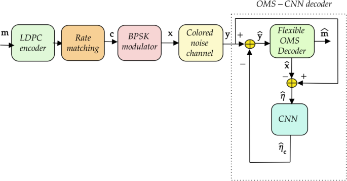
This section provides an in-depth explanation of the proposed OMS-CNN architecture, illustrated in Fig. 1. The role of the custom cost function, specifically designed for CNN optimization, and the architecture itself are discussed based on the methodology presented in⁴¹.

Proposed OMS-CNN architecture.

Full size image

OMS-CNN design flowchart

Flowchart illustrating the OMS-CNN design process.

Full size image

The OMS-CNN design process is outlined in Fig. 2, commencing at the receiver end of the communication system. The procedure involves the following sequential steps:

1. 1.

   Signal Reception and LLR Calculation: After receiving the signal (textbf{y}), the Log-Likelihood Ratios (LLRs) corresponding to the received symbols are computed, denoted as (L_{v_s}).

2. 2.

   OMS Decoder Input: The computed LLR values are then input into the OMS decoder, which generates an estimate of the transmitted symbol vector, (widehat{textbf{x}}).

3. 3.

   Channel Noise Estimation: The estimated channel noise, (widehat{varvec{eta }}), may differ from the actual noise (varvec{eta }) due to decoding errors. The relationship between the actual and estimated noise can be expressed as (widehat{varvec{eta }} = varvec{eta } + textbf{e}), where (textbf{e}) represents the noise estimation error.

4. 4.

   CNN Processing: The estimated noise, (widehat{varvec{eta }}), is then processed by a trained CNN. The CNN leverages the inherent correlation in the channel noise (varvec{eta }) to effectively suppress the error component (textbf{e}), producing an improved noise estimate, (widehat{varvec{eta }_c}).

5. 5.

   Signal Adjustment: The CNN-generated output (widehat{varvec{eta }_c}) is subtracted from the received signal (textbf{y}), resulting in an updated signal vector (widehat{textbf{y}}), expressed as:

   $$begin{aligned} widehat{textbf{y}} = textbf{y} – widehat{varvec{eta }_c} = textbf{x} + varvec{eta } – widehat{varvec{eta }_c} = textbf{x} + mathbf {r_n}, end{aligned}$$

   (18)

   where (mathbf {r_n} = varvec{eta } – widehat{varvec{eta }_c}) denotes the residual noise after CNN processing.

6. 6.

   OMS Decoding: The updated signal vector (widehat{textbf{y}}) undergoes a second round of decoding via the OMS decoder. Before this step, the LLRs are updated to (L_{{v_s}}^{(2)}), where the superscript ((2)) signifies the post-CNN processing LLR values.

The characteristics of the residual noise (mathbf {r_n}) significantly influence the updated LLR computation and the overall performance of the subsequent OMS decoding. Therefore, it is essential to train the CNN to minimize the residual noise by accurately estimating the channel noise. This is achieved using a custom cost function (mathscr {C}_{text {fading}}), as outlined in (22). By structuring the OMS-CNN process in this manner, the proposed methodology enhances channel noise estimation accuracy, leading to improved decoding performance in noisy communication environments.

CNN structure for noise estimation

Proposed CNN structure.

Full size image

The proposed OMS-CNN architecture employs a 1-D CNN, a specialized version of the traditional CNN, designed for processing one-dimensional data⁴². Figure 3 illustrates the detailed structure, including the number of layers, kernel sizes, and feature maps for each layer. Before training the network, specific parameters are initialized. Unlike conventional CNN architectures, this design does not utilize fully connected, dropout, or max pooling layers, as the input and output sizes remain identical, maintaining a consistent representation throughout. The CNN consists of four convolutional layers. Each 1-D convolutional layer applies filters to the input data, which is represented as a one-dimensional sequence. After OMS decoding, the estimated channel noise (widehat{varvec{eta }}) is fed into the CNN as a 1-D vector with dimensions (3808 times 1). Each convolutional layer contains several learnable filters (kernels), which are small segments of weights that move along the input data, performing element-wise multiplication and summation. This operation extracts specific features from the input, producing a new output array called a feature map. Each convolutional layer typically has multiple filters, allowing it to detect different features or patterns. The feature map for the (mathfrak {b})-th filter in the (mathfrak {a})-th layer, denoted as (mathcal {F}_{mathfrak {a}, mathfrak {b}}), is computed as follows:

1. 1.

   First Layer:

   $$begin{aligned} mathcal {F}_{1,mathfrak {b}} = text {ReLU}(mathbb {K}_{1,mathfrak {b}} * widehat{varvec{eta }} + mathcal {B}_{1,mathfrak {b}}), end{aligned}$$

   (19)

   where (mathbb {K}_{1,mathfrak {b}}) is the (mathfrak {b})-th kernel of the first layer, and (mathcal {B}_{1,mathfrak {b}}) is the corresponding bias.

2. 2.

   Intermediate Layers: For subsequent layers, the feature map is computed as:

   $$begin{aligned} mathcal {F}_{mathfrak {a},mathfrak {b}} = text {ReLU}(mathbb {K}_{mathfrak {a},mathfrak {b}} * mathcal {F}_{mathfrak {a}-1} + mathcal {B}_{mathfrak {a},mathfrak {b}}), end{aligned}$$

   (20)

   where (mathcal {F}_{mathfrak {a}-1}) is the feature map output from the previous layer.

3. 3.

   Final Layer: In the last layer, the estimated channel noise (widehat{varvec{eta }_c}) is computed as:

   $$begin{aligned} widehat{varvec{eta }_c} = mathbb {K}_{L} * mathcal {F}_{L-1} + mathcal {B}_{L}, end{aligned}$$

   (21)

   where (mathbb {K}_{L}) and (mathcal {B}_{L}) represent the kernel and bias for the final layer.

In these expressions, (mathbb {K}_{mathfrak {a},mathfrak {b}}) is the (mathfrak {b})-th kernel in the (mathfrak {a})-th layer, and (mathcal {B}_{mathfrak {a},mathfrak {b}}) is the corresponding bias. After applying convolution, a non-linear activation function, typically Rectified Linear Unit (ReLU)⁴³, is used. The output of each convolutional layer is a set of feature maps that indicate the presence of specific patterns or features detected by the filters. This convolution operation is repeated for each filter in the layer, producing multiple feature maps that capture various aspects of the input data.

Proposed custom cost function for fading channels

In this section, we propose a custom cost function tailored specifically for Rician, Nakagami-m, and Rayleigh fading channels. This cost function is designed to optimize the CNN’s performance by considering the characteristics of these fading channels, which introduce both random amplitude and phase variations. The proposed cost function is formulated as:

Here, (Vert mathbf {r_n}Vert ^2) is the squared norm of the residual noise, defined as (mathbf {r_n} = varvec{eta } – widehat{varvec{eta }_c}), where (varvec{eta }) is the actual channel noise and (widehat{varvec{eta }_c}) is the noise estimated by the CNN. The parameter N represents the length of the codeword, and (rho) is a scaling factor. The skewness S of the estimated noise is computed as

where (r_i) is the residual noise sample and (overline{r}) is the mean of the residual noise. The kurtosis (mathcal {K}) of the estimated noise is calculated by

The theoretical kurtosis (mathcal {K}_0) specific to the fading channel depends on the fading type: for Rayleigh fading, (mathcal {K}_0 = 3); for Nakagami-m fading, it is

where m is the shape parameter of the Nakagami distribution; and for Rician fading, it depends on the (nu)-factor and can be approximated as

Finally, (lambda) is a regularization parameter, and (text {VAR}(alpha )) denotes the variance of the fading amplitude (alpha), capturing the variation due to the fading channel.

Components of the cost function:

1. 1.

   Residual Noise Minimization:

   $$begin{aligned} frac{Vert mathbf {r_n}Vert ^2}{N}. end{aligned}$$

   (27)

   This term minimizes the average residual noise power, encouraging the CNN to accurately estimate the channel noise.

2. 2.

   Normality Regularization:

   $$begin{aligned} rho left( S^2 + frac{1}{4} (mathcal {K} – mathcal {K}_0)^2 right) . end{aligned}$$

   (28)

   This term regularizes the skewness and kurtosis of the noise distribution⁴⁴. Unlike the AWGN channel, where the target is a normal distribution, the kurtosis (mathcal {K}_0) is adjusted to match the fading channel:

   • For Rayleigh fading, (mathcal {K}_0 = 3) (kurtosis of Rayleigh distribution).

   • For Nakagami-m fading, (mathcal {K}_0) depends on the fading parameter (m).

   • For Rician fading, (mathcal {K}_0) is determined by the Rician (nu)-factor.

3. 3.

   Fading Amplitude Regularization:

   $$begin{aligned} lambda cdot text {VAR}(alpha ) end{aligned}$$

   (29)

   This term penalizes large variations in the fading amplitude (alpha). The variance of (alpha) quantifies how much the amplitude deviates from its mean. Minimizing this term encourages more accurate estimation of the fading amplitude.

Steps for implementing the custom cost function:

1. 1.

   Compute Residual Noise: Calculate the difference between the actual and estimated noise for each sample.

2. 2.

   Calculate Skewness and Kurtosis: Compute the skewness and kurtosis of the estimated noise, adjusting (mathcal {K}_0) based on the specific fading channel (Rayleigh, Nakagami-m, or Rician).

3. 3.

   Compute Fading Amplitude Variance: Estimate the fading amplitude (alpha) and compute its variance.

4. 4.

   Incorporate into Cost Function: Apply the defined cost function (mathscr {C}_{text {fading}}) to compute the loss during each training step.

5. 5.

   Optimize: Use an Adam optimization algorithm to minimize the residual noise and optimize the network weights during training.

Advantages of the proposed cost function:

• Channel-Specific Adaptation: By adjusting the kurtosis to match the characteristics of the fading channel, the cost function is more suitable for handling the variability introduced by Rician, Nakagami-m, and Rayleigh channels.

• Fading Amplitude Control: The inclusion of fading amplitude variance regularization helps improve the accuracy of signal estimation under fading conditions.

• Normality Enforcement: Regularizing skewness and kurtosis ensures the estimated noise distribution remains well-behaved, leading to improved performance in noise-affected environments.

This custom cost function is designed to improve noise estimation and decoding performance under realistic fading conditions encountered in wireless communication systems, making it suitable for Rician, Nakagami-m, and Rayleigh fading channels.

Noise sample generation for CNN training

In this section, we present a method for generating realistic noise samples tailored for CNN training in fading channels. The noise generation process is crucial for training the network to estimate and mitigate noise effects in different environments. The general formula for generating noise samples is given by:

Here, (varvec{eta }) denotes the noise sample vector, (mathcal {T}) represents the channel correlation matrix that models the correlation properties of the noise, and (varvec{eta }_f) is a vector of specific fading channel samples. The matrix (mathcal {T}) encapsulates how noise samples are correlated due to the communication channel’s characteristics. These noise samples are then used to train the CNN, allowing it to learn and adjust to the specific noise conditions. By exposing the network to these noise samples, the CNN becomes better equipped to estimate and suppress noise effectively, leading to enhanced performance in signal decoding. This method enables the network to handle various noise patterns, contributing to improved accuracy and reliability in wireless communication systems.

Convolutional processing in CNNs: focus on noise patterns

In Convolutional Neural Networks (CNNs), the convolution operation on colored noise data involves sliding a filter (kernel) over the input noise vector. At each step, the dot product between the filter’s weights and the corresponding segment of the input data is computed. Let the filter contain weights ([w_1, w_2, dots , w_k]) of size (k), and at time step (t), it covers the segment ([eta _{t-k+1}, dots , eta _t]). The convolution at this point is given by:

The resulting value (V_t) forms one entry in the feature map. Following the convolution, the ReLU activation function is applied:

This process of convolution followed by ReLU activation enables detection of regions with strong autocorrelation in the time series. For an auto-regressive (AR) series with a correlation coefficient (beta) close to 1, consecutive values are likely similar and positive. If the filter weights are designed to recognize such patterns (e.g., positive weights), the convolution (V_t) will produce a significant positive value when (eta _t) and (eta _{t-1}) are both positive, which will pass through the ReLU. As a result, (L_t) will be large in areas with high positive autocorrelation, highlighting those regions in the feature map.

Simulation setup and training methodology

The design validation employs the 5G LDPC code, specifically the BGM1 form with a base code rate of (R = 1/3) and a codeword length of (N = 3808). TensorFlow, Google Colab, and MATLAB were utilized to construct the simulation platform^45,46,47. Before training, it was necessary to generate the training data. In machine learning, generating validation data is a common practice to evaluate the network’s cost function and minimize overfitting risk. The training data were generated across different signal-to-noise ratio (SNR) levels, ranging from 0 dB to 10 dB. Each SNR level was equally represented within the total dataset. The codewords were generated using MATLAB, employing the 5G LDPC BGM1 with a base code rate of (R = 1/3) and a codeword length of (N = 3808). The LDPC matrix structure follows the standards defined by the 3rd Generation Partnership Project (3GPP) for 5G New Radio (NR). In all simulations, the offset parameter (theta) for the OMS decoder was set to 0.5, as per the optimized settings for LDPC decoding in correlated noise environments. This choice ensures better convergence of the iterative decoding process. The network was trained using a conventional mini-batch gradient descent approach. The data corresponding to each SNR level occupied an equal portion of the dataset, with each mini-batch consisting of 1200 data blocks. In each iteration, a mini-batch of training data was randomly selected to calculate the gradient. The adaptive moment estimation (Adam) optimization algorithm^48,49 was applied to determine the optimal parameters for the network. The training process continued until the loss function showed no further reduction for a prolonged duration. Table 3 lists the CNN parameters and their respective values. The bit error rate (BER) was used to assess system performance. This metric accounted for the channel’s energy efficiency using the ({E_{b}/N_{o}}) ratio at a target BER of (10^{-6}). For valid estimation, each BER measurement observed at least one hundred frame errors⁵⁰.

The parameter values of the CNN architecture—including filter dimensions, feature map counts, activation functions, optimizer choice, and the absence of padding and pooling layers—were chosen based on a combination of prior study⁵¹ and empirical tuning tailored specifically to our problem domain. The selection was carefully designed to balance performance and computational efficiency. Specifically, the chosen filter sizes 59, 24, 12, 16 and corresponding feature map counts 64, 32, 16, 1 were inspired by architectures reported in recent state-of-the-art works⁵¹ addressing similar 1D signal processing tasks, where multi-scale feature extraction is critical. We initially adopted these parameters from prior studies that demonstrated effective hierarchical feature learning without significant information loss. Unlike common CNN designs, we opted for no padding and no pooling layers to preserve the input sequence length throughout the network. Maintaining the spatial dimension was crucial for our regression task, as this design choice helps in accurately mapping input to output vectors without dimensionality reduction. The ReLU activation function and Adam optimizer were selected due to their well-established effectiveness in improving convergence speed and stability in deep learning models. To further optimize performance, we conducted systematic hyperparameter tuning experiments by varying filter sizes and feature map counts around the initial settings. The final selected parameters represent a balanced configuration that maximizes accuracy—achieving 95.8%—while maintaining computational efficiency. Finally, the Kaiming (He) initialization method was chosen to facilitate effective training with ReLU activations by mitigating the issues of vanishing or exploding gradients. In summary, the CNN parameters were guided by prior literature on similar tasks and refined through targeted empirical experiments on our dataset. These choices were validated by the achieved performance metrics and the stable convergence behavior observed during training.

Table 3 provides a comprehensive overview of the key parameters used in the CNN architecture. The network consists of four convolutional layers, each with varying filter dimensions and feature map counts. No padding or pooling layers were utilized in this design, and the activation function employed is the ReLU function. The Adam optimizer was selected for network training, and the Kaiming (He) initialization method was used for weight initialization⁵². The table also outlines the dataset sizes for training and testing, the number of epochs, and the final accuracy achieved during training. The loss function includes both residual noise minimization and regularization terms, ensuring improved noise estimation and network performance. The proposed OMS-CNN decoder does not require separate training for each channel model, as the network can generalize channel noise characteristics during training. However, channel-specific training may enhance performance due to the distinct statistical properties of Rician, Nakagami-m, and Rayleigh fading channels, including differences in amplitude, phase, correlation, skewness, and kurtosis. The custom cost function (mathscr {C}_{text {fading}}) includes kurtosis terms tailored to these channels, such as (mathcal {K}_0 = 3 + frac{6}{K+2}) for Rician fading and (mathcal {K}_0 = 3 + frac{6}{m}) for Nakagami-m fading. These variations impact residual noise and require training the CNN to adapt to specific channel conditions for optimal noise estimation and suppression. Generalized training is possible using hybrid datasets from all channel types, dynamically adjusting (mathcal {K}_0) in the cost function. While generalized models simplify deployment, they may under-perform compared to channel-specific training, which achieves better BER performance, as shown in experiments (e.g., BER of (10^{-6}) at 4.7 dB for Rician fading). For real-world 5G IoT applications, channel-specific training is recommended during development, with generalized models reserved for dynamically varying channel environments where retraining is infeasible.

The error floor performance of LDPC codes is a critical metric for assessing decoding schemes. The proposed OMS-CNN decoder demonstrates effective error floor stabilization for the given LDPC code parameters (N = 3808), (R = 1/3) under different noise correlation levels (beta). Based on the observed BER trends, the error floor stabilization threshold for the OMS-CNN decoder typically falls within (E_b/N_o) values of 4.5 dB to 5.5 dB, depending on the noise correlation. For highly correlated noise (beta = 0.9), the error floor stabilizes around (4.7 , text {dB}). With moderate correlation (beta = 0.5), this threshold increases to approximately (5.2 , text {dB}). In uncorrelated noise scenarios (beta = 0.0), the error floor stabilization occurs near (5.7 , text {dB}). These results confirm that the OMS-CNN decoder achieves robust performance, effectively mitigating noise correlation and minimizing residual errors across different channel conditions. The refined results will provide valuable insights into the decoder’s ability to address error floor challenges, particularly in 5G-enabled IoT applications where low BERs are essential.

Analyzing performance

The design’s performance in fading channels is significantly affected by three key parameters:

• Correlation coefficient (beta),

• Scaling parameter (rho), and

• Number of repetitions between the OMS and CNN stages.

Decoder performance in fading channels with correlation coefficient

In this study, we evaluate the performance of the proposed design across three types of fading channels: Rician, Nakagami-m, and Rayleigh. The SNR values at a BER of (10^{-6}) for various correlation coefficients (beta) and scalar factors (rho) are presented in Table 4. For the Rician fading channel, the proposed decoder exhibits significant performance gains, achieving an SNR of 4.7 dB when (beta = 0.9) and (rho = 0.1). As the correlation coefficient decreases to (beta = 0.5), the SNR reach to 6.3 dB, demonstrating the adaptability of the (text {(OMS-CNN)}) decoder to different correlation levels. When the correlation is absent (beta = 0), the performance converges with the traditional OMS decoder, with an SNR of 7.6 dB. For the Nakagami-m fading channel, similar trends are observed. The highest performance gain occurs at (beta = 0.9), with an SNR of 5.8 dB. As the correlation decreases to (beta = 0.5), the SNR increases to 7.1 dB. When the correlation is absent (beta = 0), the performance of the (text {(OMS-CNN)}) decoder aligns with that of the standard OMS, yielding an SNR of 8.5 dB.

In the Rayleigh fading channel, the (text {(OMS-CNN)}) decoder shows superior performance compared to the traditional OMS decoder for all tested scenarios. For high correlation (beta = 0.9), the SNR is 6.7 dB, and it increases to 8.2 dB when (beta = 0.5). The performance becomes identical to the conventional OMS decoder with an SNR of 9.7 dB when the correlation is absent. From Figs. 4, 5, 6 the findings confirm that the proposed OMS-CNN decoder effectively adapts to various fading environments and correlation levels, consistently outperforming the SPA and OMS decoders in scenarios with correlated noise. Specifically, with a correlation coefficient of (beta = 0.9), the OMS-CNN decoder demonstrated significant performance improvements, achieving gains of 2.9 dB in Rician fading, 2.7 dB in Nakagami-m fading, and 2.7 dB in Rayleigh fading, with particular effectiveness in Rician conditions. As shown in Table 4, the performance gains increase with higher correlation coefficients, confirming that the OMS-CNN decoder is well-suited to exploit channel correlation for improved decoding efficiency.

BER plot of various algorithms under correlation noise for Rician fading channel.

Full size image

BER plot of various algorithms under correlation noise for Nakagami-m fading channel.

Full size image

BER plot of various algorithms under correlation noise for Rayleigh fading channel.

Full size image

The selection of scaling factor for fading channels

In fading channel environments, the scaling factor (rho) in the custom cost function (mathscr {C}_{text {fading}}) plays a critical role in balancing two primary objectives: minimizing the residual noise power ((Vert mathbf {r_n}Vert ^2 / N)) to improve decoding performance and regularizing the statistical properties of the residual noise, such as skewness ((S)) and kurtosis ((mathcal {K})), to align with the characteristics of the fading channel. This balance is essential for the decoder to effectively mitigate noise while maintaining compatibility with the statistical distribution of fading-induced noise. Simulations reveal that small values of (rho) prioritize noise power reduction but fail to preserve the required statistical alignment, particularly in complex fading scenarios like Rician or Nakagami-m channels. This imbalance reduces the decoder’s ability to leverage the channel’s statistical characteristics, leading to suboptimal performance. Conversely, excessively high (rho) values overemphasize regularizing noise properties, which limits the suppression of residual noise power and increases decoding errors due to inadequate noise minimization.

An optimal balance is achieved with a moderate value of (rho), such as (rho = 0.3), which ensures accurate noise power minimization while maintaining alignment with fading channel properties. Empirical results demonstrate that under Rician fading conditions, a moderate (rho) achieves a bit error rate (BER) of (10^{-6}) at 4.7 dB, significantly outperforming extreme (rho) values. For instance, a very low (rho = 0.01) results in a BER of (5 times 10^{-6}), whereas a high (rho = 20) increases the BER to (7 times 10^{-3}), highlighting the importance of proper tuning. Figure 7 illustrates the performance of the proposed CNN decoder for an LDPC code under Rician fading conditions. The results show that the decoder’s performance is highly sensitive to the choice of (rho). Table 5 presents the bit error rate (BER) values for various (rho) values under the same conditions. It is evident from the table that optimal performance occurs at (rho = 0.3), achieving a BER of (10^{-6}) at 4.7 dB. This shows that, for Rician fading, a moderate (rho) value strikes the best balance between noise power reduction and maintaining the appropriate distribution.

The Table 5 also reveals that both very low and very high (rho) values lead to poorer performance. For instance, a very small (rho) of 0.01 results in a BER of (5 times 10^{-6}), while an excessively high (rho) of 20 yields a significantly worse BER of (7 times 10^{-3}). This demonstrates the need to carefully adjust (rho) based on the specific characteristics of the fading channel. These findings underscore the sensitivity of decoder performance to the selection of (rho). A well-chosen (rho) balances residual noise suppression and statistical alignment, enabling the decoder to adapt dynamically to varying fading channel conditions and achieve optimal performance in challenging communication environments.

BER plot of OMS-CNN for the best-performing (rho) values under Rician fading.

Full size image

The influence of iterations between CNN and OMS in fading channels

In the initial simulation results for fading channels, the performance of the OMS-CNN decoder was evaluated using a single iteration, denoted as (text {(OMS-CNN)}_1), for an LDPC code with a base code rate of 1/3, a codeword length of 3808, and 15 OMS iterations. The Rician fading environment is considered, which introduce additional variations in the channel characteristics. To further enhance performance in such fading conditions, multiple iterations between the CNN and OMS can be introduced. ((text {OMS-CNN})_k) represents the iteration process where (i_t) iterations are performed between the OMS decoder and the CNN. In Figure 8, at a BER of (10^{-6}), using two iterations between the CNN and OMS, denoted as (text {(OMS-CNN)}_2), results in an approximate 0.1 dB improvement in decoding performance over the single iteration (text {(OMS-CNN)}_1). This improvement is particularly important in fading channels, where the noise characteristics vary more significantly compared to AWGN channels. It is also observed that after four iterations, denoted as (text {(OMS-CNN)}_4), further performance improvement of 0.3 dB. At this point, the CNN reaches its full capability in mitigating the residual noise caused by the fading effects. Beyond this, additional iterations do not provide significant performance gains because the CNN has reached its limit in compensating for the complex fading-induced noise. In summary, while increasing the number of iterations between CNN and OMS improves performance in fading channels, particularly at lower BERs, the returns diminish after four iterations.

BER plot of various iterations between OMS-CNN design for Rician fading.

Full size image

The CNN component in the OMS-CNN decoder plays a critical role in addressing the residual noise caused by fading effects. By leveraging its deep learning capability, the CNN learns to model and mitigate noise patterns, adapting effectively to varying noise profiles encountered in different fading channel environments. Specifically, the CNN refines the residual noise estimate, represented as (mathbf {r_n} = varvec{eta } – widehat{varvec{eta }_c}), where (varvec{eta }) is the actual noise and (widehat{varvec{eta }_c}) is the CNN-estimated noise. Through iterative training and noise suppression, the CNN progressively reduces the residual noise power, improving the accuracy of the log-likelihood ratios (LLRs) used in decoding. After four iterations ((text {OMS-CNN})_4), the residual noise power stabilizes, and further refinements provide diminishing BER improvements. This stabilization indicates that the CNN has reached its full capability, having captured and compensated for the complex fading-induced noise patterns. Notably, in highly correlated noise environments (beta = 0.9), the CNN demonstrates its ability to adapt to the intricate dependencies within the noise, achieving substantial gains in decoding performance. This iterative process highlights the synergy between the CNN and the OMS decoder, where the CNN dynamically adapts to channel noise characteristics, ensuring robust decoding and high efficiency in both correlated and uncorrelated noise scenarios. By fully exploiting the statistical properties of fading channels, the CNN component significantly enhances the overall decoding process within the OMS-CNN framework.

The observed diminishing improvements in BER after four iterations are specific to the code length (N = 3808) and the correlation conditions of the simulated fading channels. This behavior is influenced by the complexity of the noise patterns and the capacity of the decoder to refine residual noise. For shorter code lengths ((N < 3808)), the decoder typically reaches this limit faster, often within two to three iterations, due to the reduced noise diversity in smaller block sizes. Conversely, for longer code lengths ((N > 3808)), additional iterations may provide further BER improvements as these codes exhibit more complex noise patterns that benefit from iterative refinement. This scalability highlights the importance of tailoring the number of iterations to the specific code length and channel characteristics for optimal decoding performance.

Computational complexity: The approximate computational complexity of ((text {OMS-CNN})_{i_t}) is derived by analyzing the contributions from the OMS decoder and the CNN. The complexity of the OMS decoder for one iteration is (mathcal {O}(text {OMS}) = M times N), where (M) represents the number of parity-check equations ((approx 2576)) and (N) is the codeword length (3808).

OMS decoder complexity: For (i_t) iterations, the OMS complexity becomes:

CNN layer complexity: The CNN complexity is determined by summing the contributions of its four layers, with each layer’s complexity given by:

For the entire CNN, the total complexity for one pass is:

For (i_t) iterations, the CNN complexity is:

Combined OMS-CNN complexity: Combining the OMS and CNN contributions, the total computational complexity for ((text {OMS-CNN})_{i_t}) is:

Substituting the values:

For ({i_t} = 4) iterations, the approximate computational complexity is:

This linear scaling with ({i_t}), combined with the dominance of the CNN component, underscores the computational efficiency of the OMS-CNN decoder. Its design balances high performance with manageable complexity, making it suitable for deployment in 5G IoT applications.

Effects of different loss functions in fading channels

In fading channels, the choice of loss functions directly influences the performance of the OMS-CNN decoder. Since the task involves predicting continuous values, regression loss functions such as Mean Squared Error (MSE) and Mean Absolute Error (MAE) are commonly used⁵³. MSE measures the average squared difference between predicted and actual values:

where (eta _i) is the actual noise value, (hat{eta }_{mu }) is the predicted noise, and (N) is the size of the coded block. MSE is sensitive to outliers, which is useful in fading channels with large deviations. MAE, on the other hand, calculates the average magnitude of errors without amplifying extreme values:

Additionally, a Custom cost function (mathscr {C}_{text {fading}}) was introduced to balance the power and distribution of residual noise in fading environments. Simulations for an LDPC code with a base rate of 1/3, using Rician channel, and 15 OMS iterations, shown in Figure 9 that (mathscr {C}_{text {fading}}) provided about 0.9 dB improvement over MAE. In conclusion, the custom cost function (mathscr {C}_{text {fading}}) enhances decoding performance in fading channels, better addressing the challenges posed by noise variability compared to traditional loss functions like MSE and MAE.

BER plot of OMS-CNN design of various loss functions for Rician channel.

Full size image

Comparative study

The proposed OMS-CNN decoder introduces significant advancements over existing LDPC decoding schemes such as Iterative BP-CNN⁵¹ and CNN-Aided Post-Processing Scheme⁵⁴. Unlike⁵¹ and⁵⁴, which primarily focus on AWGN and correlated noise, OMS-CNN is explicitly designed for fading channel environments commonly encountered in 5G-enabled IoT networks, such as Rician, Nakagami-m, and Rayleigh channels. This is achieved by incorporating skewness and kurtosis regularization into its custom cost function, which aligns residual noise characteristics with fading channel properties. Additionally, OMS-CNN explicitly handles fading amplitude variations ((text {VAR}(alpha ))) for enhanced noise estimation in dynamic conditions. A key novelty of the OMS-CNN decoder is its optimization for 5G LDPC BGM1, supporting a codeword length of (N = 3808) with (R = 1/3). This ensures compatibility with modern 5G communication standards, making the decoder suitable for URLLC and mMTC applications in IoT. Furthermore, the OMS-CNN leverages the OMS algorithm, which reduces computational complexity compared to the computationally intensive BP-CNN used in⁵¹. By iteratively updating LLRs with OMS decoding and CNN-based noise suppression, OMS-CNN achieves substantial performance gains while maintaining moderate computational overhead, making it ideal for resource-constrained IoT devices.

Unlike⁵⁴, which applies a lightweight but less effective threshold-based CNN approach for post-processing, OMS-CNN is trained and tested on realistic noise models tailored to fading channels, ensuring robust performance across diverse 5G IoT environments. Simulation results demonstrate that OMS-CNN achieves a BER of (10^{-6}) at 4.7 dB under Rician fading, outperforming⁵¹ and⁵⁴, which achieve (10^{-6}) at 2.1 dB and (10^{-5}) at 3.5 dB, respectively. These results highlight OMS-CNN’s superior ability to handle fading channel conditions with lower computational demands, making it a highly relevant and efficient solution for 5G IoT applications, such as smart cities, industrial automation, and connected healthcare systems. The comparative performance of OMS-CNN and existing schemes^51,54 is summarized in Table 6.

BER plot of various code rates for N = 3808 for Rician fading channel.

Full size image

Rate matching

Rate matching techniques that allow decoders to handle punctured (rate-increased) or shorted (rate-decreased) versions of the mother code without significant loss in decoding performance^55,56,57. This involves algorithms that can reconfigure based on the presence or absence of bits. For 5G NR-compliant QC LDPC code, the recommended decoder provides runtime flexibility and can decode received messages corresponding to code rates (R=) 1/3, 2/5, 1/2, 2/3, 3/4, 5/6, and 8/9 with base codeword length N = 3808. Furthermore, Figure. 10 indicates that the performance is enhanced for lesser code rates, such as 1/3 and 2/5. In contrast, this performance experiences a decline when the code rate is increased, as evidenced by the 5/6 and 8/9 codes. The BER plot of the multiple code rates for N = 3808 when (beta) = 0.9 and (rho) = 0.3 was applied to (hbox {(OMS-CNN)}_1).

1. Banda, L., Mzyece, M. & Mekuria, F. 5g business models for mobile network operators–a survey. Ieee Access 10, 94851–94886 (2022).

   Article  Google Scholar 

2. Diao, Z. & Sun, F. Application of internet of things in smart factories under the background of industry 4.0 and 5g communication technology. Math. Problems Eng. 2022, 4417620 (2022).

   Article  Google Scholar 

3. Popovski, P., Trillingsgaard, K. F., Simeone, O. & Durisi, G. 5g wireless network slicing for embb, urllc, and mmtc: A communication-theoretic view. Ieee Access 6, 55765–55779 (2018).

   Article  Google Scholar 

4. Ramirez, R., Huang, C.-Y. & Liang, S.-H. 5g digital twin: A study of enabling technologies. Appl. Sci. 12, 7794 (2022).

   Article  Google Scholar 

5. Jiang, X. et al. Packet detection by a single ofdm symbol in urllc for critical industrial control: A realistic study. IEEE J. Selected Areas in Commun. 37, 933–946 (2019).

   Article  Google Scholar 

6. Noor-A-Rahim, M. et al. Wireless communications for smart manufacturing and industrial iot: Existing technologies, 5g and beyond. Sensors 23, 73 (2022).

   Article  PubMed  PubMed Central  Google Scholar 

7. Wang, N. et al. Satellite support for enhanced mobile broadband content delivery in 5g. In 2018 IEEE International Symposium on Broadband Multimedia Systems and Broadcasting (BMSB), 1–6 (IEEE, 2018).

8. Mahmood, A. et al. Industrial iot in 5g-and-beyond networks: Vision, architecture, and design trends. IEEE Trans. Indust. Inform. 18, 4122–4137 (2021).

   Article  MathSciNet  Google Scholar 

9. Krummacker, D., Veith, B., Fischer, C. & Schotten, H. D. Analysis of 5g channel access for collaboration with tsn concluding at a 5g scheduling mechanism. Network 2, 440–455 (2022).

   Article  Google Scholar 

10. Sanchez, J. D. V., Urquiza-Aguiar, L. & Paredes Paredes, M. C. Fading channel models for mm-wave communications. Electronics 10, 798 (2021).

    Article  Google Scholar 

11. Tera, S. P. et al. Cnn-based approach for enhancing 5g ldpc code decoding performance. IEEE Access (2024).

12. Tera, S. P., Chinthaginjala, R., Natha, P., Ahmad, S. & Pau, G. Deep learning approach for efficient 5g ldpc decoding in iot. IEEE Access (2024).

13. Natha, P. & RajaRajeswari, P. Advancing skin cancer prediction using ensemble models. Computers 13, 157 (2024).

    Article  Google Scholar 

14. Karthiga, R. et al. A novel exploratory hybrid deep neural network to predict breast cancer for mammography based on wavelet features. Multimed. Tools Appl. 83, 65441–65467 (2024).

    Article  Google Scholar 

15. Renugadevi, M. et al. Machine learning empowered brain tumor segmentation and grading model for lifetime prediction. IEEE Access 11, 120868–120880 (2023).

    Article  Google Scholar 

16. Gupta, A. K., Srinivasulu, A., Oyerinde, O. O., Pau, G. & Ravikumar, C. Covid-19 data analytics using extended convolutional technique. Interdiscip. Perspect. Infect. Diseas. 2022, 4578838 (2022).

    Google Scholar 

17. Kim, T.-H. et al. Improving cnn predictive accuracy in covid-19 health analytics. Sci. Reports 15, 29864 (2025).

    Google Scholar 

18. Kumar, N. S. et al. Harnet in deep learning approach–a systematic survey. Sci. Reports 14, 8363 (2024).

    Google Scholar 

19. Ravikumar, C. et al. Developing novel channel estimation and hybrid precoding in millimeter-wave communication system using heuristic-based deep learning. Energy 268, 126600 (2023).

    Article  Google Scholar 

20. CV, R. K. & Bagadi, K. P. Mc–cdma receiver design using recurrent neural networks for eliminating multiple access interference and nonlinear distortion. Int. J. Commun. Syst. 30, e3328 (2017).

    Article  Google Scholar 

21. Tera, S. P., Chinthaginjala, R., Pau, G. & Kim, T. H. Towards 6g: An overview of the next generation of intelligent network connectivity. IEEE Access (2024).

22. Kim, T. H., Chinthaginjala, R., Srinivasulu, A., Tera, S. P. & Rab, S. O. Covid-19 health data prediction: A critical evaluation of cnn-based approaches. Sci. Reports 15, 9121 (2025).

    Google Scholar 

23. Natha, P. et al. Boosting skin cancer diagnosis accuracy with ensemble approach. Sci. Reports 15, 1290 (2025).

    Google Scholar 

24. Chinthaginjala, R. et al. Hybrid ai and semiconductor approaches for power quality improvement. Sci. Reports 15, 25640 (2025).

    Google Scholar 

25. Kim, T.-H. et al. Enhancing cybersecurity through script development using machine and deep learning for advanced threat mitigation. Sci. Reports 15, 8297 (2025).

    Google Scholar 

26. Sreenivasulu, V. & Ravikumar, C. Fractalnet-based key generation for authentication in voice over ip using blockchain. Ain Shams Eng. J. 16, 103286 (2025).

    Article  Google Scholar 

27. Ad-Hoc chair (Nokia). Chairman’s Notes of Agenda Item 7.1.4. Channel Coding. 3GPP TSG RAN WG1 Meeting AH 2, R1-1711982, Available Online: https://portal.3gpp.org (2017).

28. Fossorier, M. P. Quasicyclic low-density parity-check codes from circulant permutation matrices. IEEE Trans. Inform. Theory 50, 1788–1793 (2004).

    Article  MathSciNet  Google Scholar 

29. Tanner, R. A recursive approach to low complexity codes. IEEE Trans. Inform. Theory 27, 533–547 (1981).

    Article  MathSciNet  Google Scholar 

30. Wiberg, N. Codes and decoding on general graphs. Ph.D. thesis, Department of electrical engineering, linköping university, Sweden, Sweden (1996).

31. Kschischang, F. R., Frey, B. J. & Loeliger, H.-A. Factor graphs and the sum-product algorithm. IEEE Trans. Inform. Theory 47, 498–519 (2001).

    Article  MathSciNet  Google Scholar 

32. Angarita, F., Valls, J., Almenar, V. & Torres, V. Reduced-complexity min-sum algorithm for decoding ldpc codes with low error-floor. IEEE Trans. Circuits and Syst.I: Regular Papers 61, 2150–2158 (2014).

    Google Scholar 

33. Tera, S. P., Alantattil, R. & Paily, R. A flexible fpga-based stochastic decoder for 5g ldpc codes. Electronics 12, 4986 (2023).

    Article  Google Scholar 

34. Rappaport, T. S. Wireless communications: principles and practice (Cambridge University Press, 2024).

    Book  Google Scholar 

35. Molisch, A. F. Wireless communications: from fundamentals to beyond 5G (John Wiley & Sons, 2022).

    Google Scholar 

36. Hajimiri, A. & Lee, T. H. A general theory of phase noise in electrical oscillators. IEEE J. Solid-State Circuits 33, 179–194 (1998).

    Article  Google Scholar 

37. Durukan, F., Güney, B. M. & Özen, A. Performance analysis of color shift keying systems in awgn and color noise environment. In 2019 27th Signal Processing and Communications Applications Conference (SIU), 1–4 (IEEE, 2019).

38. Mochizuki, K. & Uchino, M. Efficient digital wide-band coloured noise generator. Electron. Lett. 37, 62–64 (2001).

    Article  Google Scholar 

39. Lugosch, L. & Gross, W. J. Neural offset min-sum decoding. In 2017 IEEE International Symposium on Information Theory (ISIT), 1361–1365 (IEEE, 2017).

40. Tran-Thi, B. N., Nguyen-Ly, T. T., Hong, H. N. & Hoang, T. An improved offset min-sum ldpc decoding algorithm for 5g new radio. In 2021 International Symposium on Electrical and Electronics Engineering (ISEE), 106–109 (IEEE, 2021).

41. Li, Z., Liu, F., Yang, W., Peng, S. & Zhou, J. A survey of convolutional neural networks: analysis, applications, and prospects. IEEE Trans. Neural Networks Learn. Syst. 33, 6999–7019 (2021).

    Article  MathSciNet  Google Scholar 

42. Qazi, E. U. H., Almorjan, A. & Zia, T. A one-dimensional convolutional neural network (1d-cnn) based deep learning system for network intrusion detection. Appl. Sci. 12, 7986 (2022).

    Article  Google Scholar 

43. Nair, V. & Hinton, G. E. Rectified linear units improve restricted boltzmann machines. In Proceedings of the 27th international conference on machine learning (ICML-10), 807–814 (2010).

44. Thadewald, T. & Büning, H. Jarque-bera test and its competitors for testing normality-a power comparison. J. Appl. Stat. 34, 87–105 (2007).

    Article  MathSciNet  Google Scholar 

45. Abadi, M. et al. ({)TensorFlow(}): a system for ({)Large-Scale(}) machine learning. In 12th USENIX symposium on operating systems design and implementation (OSDI 16), 265–283 (2016).

46. Carneiro, T. et al. Performance analysis of google colaboratory as a tool for accelerating deep learning applications. IEEE Access 6, 61677–61685 (2018).

    Article  Google Scholar 

47. Sharma, V., Gupta, G. K. & Gupta, M. Performance benchmarking of gpu and tpu on google colaboratory for convolutional neural network. In Applications of Artificial Intelligence in Engineering: Proceedings of First Global Conference on Artificial Intelligence and Applications (GCAIA 2020), 639–646 (Springer, 2021).

48. Glorot, X. & Bengio, Y. Understanding the difficulty of training deep feedforward neural networks. In Proceedings of the thirteenth international conference on artificial intelligence and statistics, 249–256 (JMLR Workshop and Conference Proceedings, 2010).

49. Kingma, D. P. Adam: A method for stochastic optimization. arXiv preprint arXiv:1412.6980 (2014).

50. Sharma, S. K., Chatzinotas, S. & Ottersten, B. Snr estimation for multi-dimensional cognitive receiver under correlated channel/noise. IEEE Trans. Wireless Commun. 12, 6392–6405 (2013).

    Article  Google Scholar 

51. Liang, F., Shen, C. & Wu, F. An iterative bp-cnn architecture for channel decoding. IEEE J. Select. Topics Signal Process. 12, 144–159 (2018).

    Article  Google Scholar 

52. He, K., Zhang, X., Ren, S. & Sun, J. Delving deep into rectifiers: Surpassing human-level performance on imagenet classification. In Proceedings of the IEEE international conference on computer vision, 1026–1034 (2015).

53. Chahkoutahi, F. & Khashei, M. Influence of cost/loss functions on classification rate: A comparative study across diverse classifiers and domains. Eng. Appl. Artific. Intell. 128, 107415 (2024).

    Article  Google Scholar 

54. Liu, J., Kang, S., Cheng, J., Wang, J. & Huang, R. A cnn-aided post-processing scheme for channel decoding under correlated noise. In 2024 3rd International Conference on Electronics and Information Technology (EIT), 150–154 (IEEE, 2024).

55. Cui, H. et al. Design of high-performance and area-efficient decoder for 5g ldpc codes. IEEE Trans. Circuits and Syst. I: Regular Papers 68, 879–891 (2020).

    MathSciNet  Google Scholar 

56. Stark, M., Wang, L., Bauch, G. & Wesel, R. D. Decoding rate-compatible 5g-ldpc codes with coarse quantization using the information bottleneck method. IEEE Open J. Commun. Soc. 1, 646–660 (2020).

    Article  Google Scholar 

57. Wu, X., Jiang, M., Zhao, C., Ma, L. & Wei, Y. Low-rate pbrl-ldpc codes for urllc in 5g. IEEE Wireless Commun. Lett. 7, 800–803 (2018).

    Article  Google Scholar 

Download references

Authors and Affiliations

1. Department of Electronics and Electrical Engineering, Indian Institute of Technology, Guwahati, Assam, 781039, India

   Sivarama Prasad

2. School of Electronics Engineering, Vellore Institute of Technology, Vellore, Tamil Nadu, 632014, India

   Ravikumar Chinthaginjala

3. Artificial Intelligence, Software, and Information Systems Engineering Departments, Research Center for AI and IoT, AI and Informatics Faculty, Near East University, Mersin 10, Nicosia, 99138, Turkey

   Fadi Al-Turjman

4. Industrial Engineering Department, College of Engineering, King Saud University, P.O. Box 800, 11421, Riyadh, Saudi Arabia

   Shafiq Ahmad

Contributions

Sivarama Prasad Tera was responsible for the conceptualization and methodology. Ravikumar Chinthaginjala contributed to data collection, software development, and visualization. Fadi Al-Turjman provided supervision of the software, resources, and validation. Shafiq Ahmad contributed through supervision and resource provision. All authors have read and approved the final version of the manuscript.

Corresponding authors

Correspondence to Ravikumar Chinthaginjala or Fadi Al-Turjman.

Competing interests

The authors declare no competing interests.

Publisher’s note

Springer Nature remains neutral with regard to jurisdictional claims in published maps and institutional affiliations.

Open Access This article is licensed under a Creative Commons Attribution-NonCommercial-NoDerivatives 4.0 International License, which permits any non-commercial use, sharing, distribution and reproduction in any medium or format, as long as you give appropriate credit to the original author(s) and the source, provide a link to the Creative Commons licence, and indicate if you modified the licensed material. You do not have permission under this licence to share adapted material derived from this article or parts of it. The images or other third party material in this article are included in the article’s Creative Commons licence, unless indicated otherwise in a credit line to the material. If material is not included in the article’s Creative Commons licence and your intended use is not permitted by statutory regulation or exceeds the permitted use, you will need to obtain permission directly from the copyright holder. To view a copy of this licence, visit http://creativecommons.org/licenses/by-nc-nd/4.0/.

Reprints and permissions