Deep learning in photonic device development: nuances and opportunities – npj Nanophotonics

Deep learning (DL) has become increasingly popular among researchers, touted as a revolutionary disruption to optimization and modeling via rapid exploration and automated characterization. Much of this enthusiasm stems from DL’s demonstrated capabilities in other domains: convolutional neural networks have enabled high-accuracy image classification^1,2, transformers have advanced attention-based reasoning and sequence modeling^3,4, and generative models such as generative adversarial networks and variational autoencoders have enabled rapid synthesis of complex, high-dimensional data^5,6. Its success in these areas reflects its ability to deliver reliable performance where few alternative methods achieve comparable results.

Based on this success, many have applied DL in the physical sciences, often using models to act as fast surrogates for linear and non-linear field equations in areas like computational fluid dynamics and electromagnetics. These models can be used to approximate solutions to Navier-Stokes and Maxwell’s equations orders of magnitude faster than conventional solvers, making device engineering feasible at previously prohibitive scales⁷. Naturally, this success has motivated efforts to apply DL across the photonic device development (PDD) cycle as well, which spans theoretical modeling, electromagnetic simulation, optimization, and fabrication⁸. Classical direct solvers such as finite-difference time domain (FDTD), finite element method (FEM), or rigourous coupled-wave analysis must repeatedly resolve fields across finely discretized domains. However, the computational resources required for numerical solvers scale poorly as the domain and problem complexity increase. Using them as a resource within PDD optimization strategies further exacerbate these issues: local, gradient-based techniques require multiple simulations per gradient update step⁹, while global methods like evolutionary algorithms attempt to efficiently search through an exponentially large design space¹⁰. In response to these bottlenecks, DL-based frameworks have been positioned as alternatives to direct solvers, thereby enabling faster device design search and reducing overall turnover¹¹. But with these powerful new capabilities, to what extent can DL truly substitute for established methods?

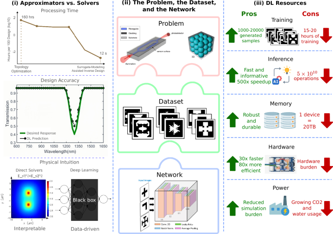
This perspective addresses this question by evaluating the current trajectory of DL in PDD, focusing on caveats that arise when comparing DL with classical methods. We emphasize three areas in particular: (1) data-driven estimations vs direct solvers; (2) dataset and model design and transferability in representing PDD problems; and (3) resource consumption of DL and numerical solvers. Figure 1 outlines these goals as well. We balance this discussion by acknowledging that DL has shown practical utility in certain scenarios, such as inverse design tasks for metasurfaces, optical switches, and antennae, along with surrogate modeling for rapid design-space exploration. We argue, however, that DL’s most sustainable and impactful contributions will arise from its integration with physics-informed approaches and hybrid strategies, such as reinforcement learning frameworks that incorporate fabrication feedback. Our goal is to present a critical yet holistic stance on where DL workflows succeed, areas of improvement, and what role they can realistically play in the design pipeline.

i) DL models promise speed and efficient searching of design spaces, taking seconds to process hundreds of designs, but lack physical intuition, suffer from slow training procedures, and lack universality. Conversely, direct solvers are accurate, grounded in physics, and convergent, but the overall computation is slow and expensive, taking hundreds of hours to process a similar number of designs. Mode analysis image adapted with permission from ref. ⁷⁵, Copyright Ansys Lumerical, 2025. Data for the processing time plot retrieved from ref. ⁷⁶, Copyright 2020 AIP Publishing and ref. ¹⁷. Design Accuracy plot adapted from ref. ⁷⁷, Copyright 2018 IEEE. ii) DL performance is often governed by the problem formulation, data quality, and the network that interprets the data. Waveguide image adapted with permission from ref. ⁷⁸, Copyright 2014 Elsevier. Photonic crystal and bandgap images adapted with permission from ref. ⁷⁹, Copyright 2019 Elsevier. Dataset and network images adapted with permission from refs. ^16,80, Copyright 2023 Optica Publishing Group and ref. ⁸¹, Copyright 2020 American Chemical Society. iii) DL is very resource intensive, often exceeding that of classical methods. Google TPU image adapted with permission from ref. ⁸².

Full size image

Deep neural networks have been proposed to model physical systems by approximating solutions to their governing partial differential equations (PDEs)¹². There are a few notable examples of trained DL models solving PDEs with computation times that are orders of magnitude faster than direct solvers, with similar accuracy. Examples include optical spectra from all-dielectric metasurfaces¹³, core-shell nanoparticles¹⁴, thermophotovoltaic cell efficiency predictions^15,16,17, etc. At a high level, this may suggest that DL models offer a viable alternative to traditional direct solvers. Closer examination, however, reveals important caveats.

Firstly, naive DL models do not enforce physical constraints a priori; instead, they infer solutions via statistical correlations learned from provided data. These models map optical parameters directly to performance metrics such as transmission, loss, or other figures of merit, and typically don’t yield interpretable intermediate quantities such as fields or mode profiles. For example, a neural network trained on simulated transmission spectra of metasurfaces may learn to associate certain geometric features with expected optical responses, but may do so without grounding those associations in any governing physics¹⁸. As a result, these models may produce nonphysical or unreliable predictions when presented with inputs that fall too far outside the distribution of their training set, exhibiting issues such as overfitting, biases, and in some contexts, adversarial injections and hallucinations. In contrast, numerical solvers rigorously enforce Maxwell’s equations and boundary conditions, producing solutions for devices with tunable accuracy¹⁹. FEM, for example, can discretize the simulation domain into meshes of small, high-order elements and solve Maxwell’s equations locally within each element^20,21. As a result, their outputs rapidly converge towards the true physical solution as the mesh is refined, allowing users to iteratively reduce numerical error in particular regions. Moreover, since Maxwell’s equations are linear in many practical problems, solvers can efficiently exploit this structure to achieve more reliable answers than data-driven models and employ the system matrices for adjoint optimization and sensitivity analysis.

Secondly, the inference speed of DL models is offset by the upfront cost of data preparation and training. Table 1 further illustrates this nuance by outlining some applications that use simulations to generate their training data. Although these models achieve low mean-squared error values, doing so requires robust, labeled training datasets generated by thousands of full-wave simulations, often using FDTD or FEM- the same direct solvers DL aims to replace. Thus, for a small number of design evaluations, the total computational cost of DL models could approach or even exceed that of using solvers directly. On the other hand, the cost of using direct solvers is mostly confined to the time required to set up the simulation and the computation time. Furthermore, especially in forward problems, the MSE only quantifies agreement with the training data, not necessarily with experimental measurements. Selecting an appropriate model structure and training strategy that accurately captures the physics is a significant challenge, especially in the absence of strong physical biases. Direct solvers utilize a range of strategies to minimize simulation overhead, including custom user interfaces in place of scripting, GPU backend accelerators, and high-performance computing workflows²². These are often complemented by specialized dataflow architectures (e.g., pipelined GPU or FPGA implementations), spectral scaling techniques for multi-frequency analysis, and domain decomposition methods, which enable efficient parallelization across distributed computer nodes.

Much of the early appeal of DL in photonics lay in its potential to bypass costly simulations by learning to emulate solvers. However, these proof-of-concept studies prioritized feasibility over practicality in a difficult domain, leading to a lack of expressive datasets that could meaningfully support the application of DL to PDD. This scarcity pushed researchers to train DL models on curated, task-specific datasets, e.g., gold patterns on glass substrates for generative adversarial networks²³ and analytical expressions for Equation Learner networks²⁴. Although these efforts were valuable, the resultant datasets were limited in size and scope, making them insufficient for training models to generalize across broader PDD applications. This contrasted with the vast, diverse datasets available for natural language processing applications, which underpin the success of commercial chatbots and large language models^25,26. A benefit of using direct solvers is that many numerical techniques are generic enough to handle multiple material properties within a large domain without additional finetuning. However, DL models need to be trained properly on several applicable domains for them to generalize well.

This prompts a broader question: is it possible to achieve more capability with less data? Full-wave simulations may produce relatively small datasets, which could be extended to broader contexts through data augmentation. If the dataset consists of images, for example, simple augmentation techniques such as rotations, flips, and crops can increase the number of available samples in the dataset while still preserving the data²⁷. Beyond these basic methods, generative models can be used to further expand datasets or introduce variability in underrepresented regions of the design space²⁸. However, physical properties still need to be considered during data augmentation, especially in problems sensitive to spatial symmetries or directional field behavior, such as beam steering or mode conversion. Without explicit enforcement, simple augmentation does not inherently satisfy these constraints and could produce non-physical field solutions that violate conservation laws. Moreover, some transformation schemes could introduce anomalies that do not reflect the underlying physics of the problem, rendering them ineffective for extrapolating beyond known patterns. Even after increasing the dataset to an acceptable size for the model, obtaining a fully expressive training set that covers all design permutations remains an intractable problem. In fact, in high-dimensional design spaces, interpolation may correspond to extrapolation beyond the training distribution, which is reflected by the limited coverage of the design space itself²⁹. For instance, the dataset for the first example mentioned in Table 1 reportedly only covered about 0.0022% of possible designs¹³.

This shows that as long as DL frameworks remain primarily data-driven, they remain vulnerable to such domain mismatch errors, unlike direct solvers. This raises the need for data efficiency, or maximizing the framework’s inferential value per unit of data³⁰ Evidently, the choice of architecture is strongly coupled to the complexity of the problem’s design space. Problems defined by a low-dimensional parametric input and few geometric variables, such as periodic metasurfaces, can be sufficiently described using a multilayer perceptron or a convolutional neural network. This is because the mapping between the few geometric variables and the output spectrum, while complex, is relatively smooth and well-behaved. However, for more complex problems such as electromagnetic scattering, optical circuit switchers, or modeling crystal structures, these standard architectures may fall short. A key reason for this is spectral bias, where neural networks have been shown to favor learning low-frequency components and struggle with highly oscillatory solutions (also known as spectral bias)³¹. This has driven the development of more specialized models. For example, to better represent the phase and amplitude of electromagnetic waves, complex-valued neural networks have been used to directly model the fields in scattering problems, providing a more natural fit for the physics³². Graph neural networks can operate on arbitrary meshes of FDTD solvers to learn local physical interactions in a flexible, size-invariant manner, making them ideal for modeling non-trivial topologies³³. These examples illustrate a clear trend: increasing data efficiency not just through more data, but by embedding structural (and possibly, physical) priors directly into the model’s architecture.

In building such data efficient DL models, their specialized nature could limit transferability, as small changes to the problem or dataset may require regenerating data or retraining the model³⁴. Traditional solvers handle changes in the problem definition through adaptive meshing or refined time steps, whereas fixed-size neural networks may not be as flexible. DL models must balance physical accuracy with transferability to ensure their usefulness. Consequently, dataset design and augmentation strategies must be tailored to the structural and physical constraints of each system to ensure meaningful extrapolation. Even still, these approaches may fall short of an accurate, generalizable technique and would require significantly more data and architectural complexity to achieve direct solver-level accuracy³⁵. Others have proposed physics-informed regularization by incorporating governing physics, such as Maxwell’s equations and conservation laws, directly into the loss function. These ideas have coalesced into a more formal framework: physics-informed neural networks (PINNs), which attempt to reconcile data-driven learning with first-principles modeling by integrating physical laws into the network architecture and training.

Case study: physics-informed neural networks (PINNs)

First introduced by Raissi et al. PINNs do two very important things. Firstly, they approximate solutions to the governing PDEs of a problem. They evaluate PDE residuals at collocation points and enforce boundary/initial conditions through their loss function³⁶. For example, in structural dynamics, physics-informed long short-term memory networks have been used to model nonlinear systems by embedding physical constraints such as equations of motion and hysteresis into the training loss³⁷. By association, PINNs show promise in handling irregular geometries, localized physics, and rapidly varying solutions. Secondly, PINNs are more data efficient due to their regularization losses, making them ideal for training on smaller datasets, such as forecasting long time-domain signals using short-sequence inputs in terahertz spectroscopy³⁸. By pretraining on low-fidelity data and fine-tuning with minimal high-fidelity data, these models efficiently generalize across diverse physical systems. Pretrained PINNs can also perform random sampling via coordinate-based networks, making them appealing for some forward problems and higher dimensional PDEs, like Poisson’s equation. They also enable accurate and cost-effective modeling across a range of photonic systems³⁹. PINNs can also be used to find unknown parameters of a known PDE from observational data: akin to an inverse problem⁴⁰.

Although PINNs and their applications are innovative and promising, traditional numerical solvers continue to outperform them in both solution time and accuracy. This has been demonstrated in benchmark comparisons involving Poisson’s equation, the Allen-Cahn equation, and the hyperbolic semilinear Schrödinger equation³⁹. Additionally, the transferability of PINNs is constrained by their boundary conditions, which must be explicitly encoded during the training phase⁴¹. Should the boundary conditions change later—to simulate a different incident angle or boundary reflectivity in a metasurface, for example—a new network must be trained from scratch, or the conditioned information has to be used as input. Further, PINNs require the user to make explicit choices about how the governing physics are represented, such as selecting which formulation of Maxwell’s equations to enforce during training. Even for problems governed by the same physical laws, different formulations can yield different outcomes, making the model’s performance sensitive to these manual decisions²¹. Lastly, PINNs suffer from a similar curse of dimensionality as observed in regular DL models. Namely, reducing generalization error requires exponentially more training points and network capacity, making PINNs impractical as dimensionality grows⁴¹. This situation is nuanced, however; conventional direct solvers such as FEM are also affected by the curse of dimensionality⁴². Even simulating processes like hyperplasticity, which are not usually deemed expensive, can become intractable as the design space grows sufficiently large. As these costs begin to compound, it becomes critical to assess the computational overhead associated with DL models and direct solvers, and whether the performance gains they offer justify the expense.

Beyond the costs of data generation and augmentation, the models themselves impose significant computational demands for training and evaluation. To illustrate these requirements, we consider recent frameworks developed for thermophotovoltaic cell design. Each of the developed models consists of about 4 million learnable parameters trained on a dataset of 12,000 designs, originally derived from FDTD simulations. This would constitute about 5 × 10¹⁰ basic operations per epoch for 10,000 epochs, without considering the surrogate model parameters or additional computations. In practice, modern generative models, such as diffusion models, can take anywhere up to 15 h to train on several GPUs running in parallel¹⁷. Since training cost scales with the dataset size and model parameters, doubling them leads to roughly a fourfold increase in total cost. Extending this to higher-order problems, this leads to a fourth-order increase in overall computational complexity⁴³.

This is not necessarily detrimental; hardware has significantly improved to adapt to these requirements by introducing more floating point operations per second. Google’s tensor processing units, specialized for deep neural networks, demonstrate a 15–30× improvement in throughput compared to contemporary CPUs and GPUs, while also achieving 30–80× higher energy efficiency⁴⁴. These improvements are substantial, but they also reveal a critical dependency: much of DL’s current progress stems from training larger models on faster hardware at increasing power and natural resource cost. One study demonstrated that three years of model development is comparable to a tenfold increase in hardware capabilities⁴³.

Sometimes, these costs can be justified when training is amortized over large volumes. For example, a physics-driven neural solver for Maxwell’s equations (MaxwellNet) required 37–63 h of training on GPUs, but simulated new scenarios in 6.4 ms, about ~625× faster than a commercial FEM solver like COMSOL Multiphysics, which took about 4 s using the same hardware¹¹. In such cases, the upfront investment in training enables rapid inference later. Otherwise, the burden of model training can be reduced through compression techniques, such as dropout, pruning, and PINN regularization, which can eliminate parameter counts and training time. However, they often require repeated fine-tuning and may offer diminishing returns when applied to already efficient models^45,46. In such cases, smaller machine learning models that do not rely on deep neural architectures, such as statistical learning methods, may outperform deep learning methods in generating high-quality images for various optical problems⁴⁷.

A direct numerical solver, on the other hand, may be more resource-effective than training a model from scratch if only a handful of simulations are needed. Classical electromagnetic solvers can parallelize across CPU cores or distributed memory nodes to yield substantial speedup compared to a single core for photonic benchmarks⁴⁸. Additionally, for a sufficiently fine grid, FDTD simulations only require the field from the previous time step to approximate the next, thereby making them more memory-efficient for larger systems with higher volumes at the cost of computation time. This helps towards mitigating problems of numerical dispersion over large propagation distances⁴⁹. That being said, numerical methods are not exempt from computational limits. For example, simulating a 100 μm² photonic device at fine resolution could require up to 20,000 compute hours (and 20TB of memory), which is only feasible on high-performance clusters¹². Volume integral methods reduce the simulation volume by solving Maxwell’s equations in integral form, but discretization (e.g., for Faraday’s law) still introduces local dependencies that increase computational overhead²⁰.

Naturally, these computational burdens translate into energy and environmental costs as well. For instance, training a single large-scale transformer model has been estimated to emit as much CO₂ as five American cars over their lifetimes^50,51, with growing attention to water and power consumption in large GPU clusters^52,53. While DL in PDD does not yet approach these scales, the lesson is cautionary: applying DL indiscriminately risks creating unnecessary environmental and resource footprints. Ultimately, both DL and numerical solvers entail trade-offs in computational cost, time, and environmental impact. These trade-offs suggest that DL could provide powerful advantages in certain scenarios, which are explored in the next section.

While the trajectory of PDD increasingly points towards the integration of DL frameworks, it is clear that they will not outright replace traditional solvers for the foreseeable future. At the very least, numerical solvers will likely always be the gold-standard for physical interpretation and accuracy. Of course, this does not mean that DL has no role to play. Emerging research shows that DL models work well in situations with several unknowns, such as problems with large, continuous design spaces, large amounts of data, slow function evaluation times, and/or non-trivial tolerance requirements⁵⁴. These conditions are already prevalent in inverse design problems, where mapping optical behavior to device geometry is a one-to-many problem and inherently ill-posed^25,55. Figure 2 illustrates the evolution of DL from early inverse design methods, such as genetic algorithms and adjoint shape optimization in electromagnetic design⁹, toward data-driven strategies.

Inverse design was largely based on genetic algorithms and adjoint optimization until GANs offered a DL-driven method. From there, DL-augmented optimization methods grew in popularity, leading to the plethora of options we have today. Genetic algorithms (2007) adapted with permission from ref. ¹⁰, Copyright 2007, Optical Society of America. Adjoint electromagnetic optimization (2013) adapted with permission from ref. ⁹, Copyright 2013, Optical Society of America. Generative adversarial networks (2018) adapted with permission from ref. ²³, Copyright 2018 American Chemical Society. PINNs adapted with permission from ref. ⁸³, Copyright 2020 CIMNE, Barcelona, Spain. RL and Fab-in-the-Loop adapted with permission from ref. ⁶⁸, Copyright 2023 The Authors, used under the Creative Commons License.

Full size image

Traditional inverse design methods, such as topology optimization, which includes a combination of evolutionary algorithms with adjoint optimization, must search the vast design space associated with such problems exhaustively- often at a high computational cost. In this regard, one of the most prominent roles of DL models today is as surrogate models: data-driven approximations that can learn complex mappings between structure and response directly from simulated or experimental datasets, thereby circumventing many of the constraints inherent to rule-based optimization. Early approaches used neural networks trained on large datasets of forward-simulated spectra to predict corresponding structural parameters and vice-versa^56,57. The versatility of this paradigm is evident in its application across a diverse range of photonic systems, from free-form metasurfaces to waveguide components. Recent demonstrations show deep neural networks being applied to the inverse design of all-optical plasmonic switches and fiber Bragg gratings, achieving accurate prediction of spectral responses using a significantly lesser number of samples^58,59.

To further address the one-to-many challenge, the field has moved towards looking at generative models. DL frameworks and surrogates based on compressing the design space, such as with variational autoencoders. These provide valuable solutions by learning a lower-dimensional latent representation of the design space that is more computationally tractable¹⁵. By conditioning the model on desired optical or material properties, they can generate many diverse geometries that satisfy the same target response. To further improve the regularization of variational autoencoders to be physics-informed, we can consider generative or conditional generative adversarial networks, which rely on adversarial learning to produce sharp, realistic outputs without requiring explicit assumptions about the underlying data distribution^60,61. More recently, diffusion models have been gaining a lot of traction because they offer better mode coverage and improved sample diversity by refining outputs through a denoising process⁶². As likelihood-based models, they can estimate the confidence or uncertainty of each generated sample, and are typically more robust to hyperparameter choices. These features make them a viable choice for complex and multimodal inverse design problems⁶³.

Neural operators extend this idea further through discretization invariance, where a learned mapping is defined over continuous function spaces rather than a fixed discretization. This is especially powerful for PDE-based physics, since the operator being learned is the solution map from inputs (e.g., material distribution or boundary conditions) to fields. In effect, the operator can help improve model generalization and transferability across different numerical solutions, meshes, or resolutions⁶⁴. For instance, the Fourier Neural Operator can be used to design complex 3D structures with fewer simulations than full-wave methods, while preserving practical accuracy. This directly tackles the problem of limited transferability and moves towards data efficiency as well. As an extension, graph kernel operators represent domains as graphs, where the nodes and edges can model local or nonlocal dependencies, thereby enabling operator learning in irregular or unstructured geometries⁶⁵. Further, geometry-inspired neural operators can take the strengths of the prior two methods along with physical awareness of the system to enable accurate out-of-distribution predictions⁶⁶.

The usefulness of these surrogate models goes beyond initial device optimization to support key engineering tasks, such as tolerance analysis, where a device’s robustness is evaluated by simulating its performance across various geometric changes. This is clear in applications like antenna engineering, where a design must achieve performance goals and withstand manufacturing imperfections. A fast surrogate can be trained on a limited number of full-wave antenna simulations, then instantly evaluate thousands of design variations, enabling a “robustness score” to be calculated for candidate designs. The design algorithm can automatically identify solutions by co-optimizing robustness with performance, thus finding options that are both high-performing and practical to manufacture⁶⁷.

A recent promising area of research for DL is fab-in-the-loop reinforcement learning, which incorporates experimental feedback directly into the optimization loop. This framework operates by assigning rewards to outcomes so that the DL model learns to generate increasingly optimal designs, e.g., grating couplers⁶⁸. The algorithm begins with a traditionally optimized design and then generates a batch of device variants across many parameters. The designs are fabricated and measured, and the resultant dataset is used to retrain the model. The process is iterated, and the best-performing fabricated designs are used as the seed for the next generation. This framework allows the reinforcement learning algorithm to converge toward highly performant, often unintuitive designs that outperform those produced by conventional methods. By accounting for real fabrication conditions, RL both improves design fidelity and significantly reduces reliance on slow, high-fidelity simulations.

However, these methods still require more physical grounding. Hybrid solvers address this concern by combining DL models with traditional physics-based optimization methods. A generative DL model proposes device geometries based on target specifications, while an adjoint electromagnetic solver guides training via backpropagation using physical gradients. This form of learning enables the model to directly learn the geometry-response relationship and can achieve high-efficiency designs with reduced computational cost⁵⁵. These frameworks could benefit data efficiency by focusing the model’s inference on the physical relationship between device geometry and response directly through electromagnetic simulations⁶⁹.

PINNs can help take this idea further. They have been applied to inverse metamaterial scattering problems, such as determining effective medium properties. They have also been used to retrieve spatial distributions of electric permittivity from scattering data of nanostructured clusters arranged in periodic or aperiodic geometries. These results have been validated against FEM simulations, underscoring PINNs’ potential for accurate and efficient solutions in low-data regimes^70,71. Building on this hybrid model-like structure, PINNs are poised to integrate with reinforcement-learning methods to enhance fabrication control by incorporating real-time data and physical constraints, leading to more reliable and precise device designs. Generally, advances in PINN theory are expected to broaden their applicability across diverse PDEs and deepen the integration of physical knowledge into model architectures.

Ultimately, the path forward is a strategic, problem-dependent integration of the approaches listed above. Enabling such a strategy, however, requires a crucial step: the development of community benchmarks to allow for fair and quantitative comparisons between methods. The FAIR (Findable, Accessible, Interoperable, Reusable) Principles offer the practical framework to build these resources. Making datasets Findable through persistent digital identifiers and Accessible via open-source, standardized protocols ensures that the entire community can locate and retrieve the same benchmark data from a variety of sources and preventing them from becoming lost or inaccessible. Ensuring the data is Interoperable through common file formats and useful metadata is the critical step that enables direct comparison of different model architectures, which is currently lacking, as shown in previous sections. Finally, making data reusable with clear licensing and documentation on their utility and application allows new research to be built upon, verified, and extended, accelerating progress for the entire field⁷².

This call for a more unified approach is already being answered. Recent initiatives, such as the proposed MAPS infrastructure, aim to create an open-source, standardized platform for exactly this purpose. By providing shared dataset acquisition frameworks and unified training and evaluation metrics, such platforms represent a critical step toward building the robust, collaborative ecosystem needed to truly advance and validate new DL models in photonics⁷³.

Deep learning is not a blanket solution for PDD problems, and efforts to use it as a drop-in replacement for conventional solvers often overlook limitations in data-driven methods when they predict physics for data outside of the training set domain. DL’s strengths lie in large-data applications where the amortization of several direct solver runs eventually overcomes simulation times, such as when generating design candidates in optimization algorithms or accelerating exploration when coupled with domain knowledge⁸. A promising path forward is to strategically integrate DL where it adds clear value: through hybrid pipelines, physics-informed modeling, and data-efficient architectures tailored to the realities of the problem. To fully realize this potential, the community must work toward addressing the methodological and conceptual limitations outlined in this perspective, especially those concerning data, generalization, and physical fidelity. That said, as these models grow more capable of embedding physical laws and constraints directly into their structure, their usefulness may shift from mere acceleration to deeper understanding through symbolic methods, enabling design and discovery workflows that are both faster and fundamentally smarter.

1. Krizhevsky, A., Sutskever, I. & Hinton, G. E. ImageNet classification with deep convolutional neural networks. Commun. ACM 60, 84–90 (2017).

   Article  Google Scholar 

2. 1. He, K., Zhang, X., Ren, S. & Sun, J. Deep Residual Learning for Image Recognition. in 2016 IEEE Conference on Computer Vision and Pattern Recognition (CVPR) 770–778 (IEEE, Las Vegas, NV, USA, 2016). https://doi.org/10.1109/CVPR.2016.90.

3. Vaswani, A. et al. Attention is All you Need. in Advances in Neural Information Processing Systems 30 (eds. Guyon, I. et al.) 6000–6010 (Curran Associates, Inc., 2017).

4. OpenAI et al. GPT-4 Technical report. http://arxiv.org/abs/2303.08774 (2024).

5. Goodfellow, I. et al. Generative adversarial networks. Commun. ACM 63, 139–144 (2020).

6. Kingma, D. P. & Welling, M. Auto-encoding variational bayes. http://arxiv.org/abs/1312.6114 (2022).

7. Brunton, S., Noack, B. & Koumoutsakos, P. Machine learning for fluid mechanics. Annu. Rev. Fluid Mech. 52, 477–508 (2020).

   Article  ADS  MathSciNet  Google Scholar 

8. Chen, Y. et al. Machine-learning-assisted photonic device development: a multiscale approach from theory to characterization. Nanophotonics. https://doi.org/10.1515/nanoph-2025-0049 (2025).

9. Lalau-Keraly, C. M., Bhargava, S., Miller, O. D. & Yablonovitch, E. Adjoint shape optimization applied to electromagnetic design. Opt. Express 21, 21693 (2013).

   Article  ADS  Google Scholar 

10. Goh, J., Fushman, I., Englund, D. & Vučković, J. Genetic optimization of photonic bandgap structures. Opt. Express 15, 8218 (2007).

    Article  ADS  Google Scholar 

11. Lim, J. & Psaltis, D. MaxwellNet: physics-driven deep neural network training based on Maxwell’s equations. APL Photonics 7, 011301 (2022).

    Article  ADS  Google Scholar 

12. Kang, C. et al. Large-scale photonic inverse design: computational challenges and breakthroughs. Nanophotonics 13, 3765–3792 (2024).

    Article  ADS  Google Scholar 

13. Nadell, C. C., Huang, B., Malof, J. M. & Padilla, W. J. Deep learning for accelerated all-dielectric metasurface design. Opt. Express 27, 27523 (2019).

    Article  ADS  Google Scholar 

14. Vahidzadeh, E. & Shankar, K. Artificial neural network-based prediction of the optical properties of spherical core-shell plasmonic metastructures. Nanomaterials 11, 633 (2021).

    Article  Google Scholar 

15. Wilson, B. A. et al. Machine learning framework for quantum sampling of highly-constrained, continuous optimization problems. Appl. Phys. Rev. 8, 041418 (2021).

    Article  ADS  Google Scholar 

16. Kudyshev, Z. A., Kildishev, A. V., Shalaev, V. M. & Boltasseva, A. Machine learning-assisted global optimization of photonic devices. Nanophotonics 10, 371–383 (2020).

    Article  ADS  Google Scholar 

17. Bezick, M. et al. PearSAN: a machine learning method for inverse design using Pearson correlated surrogate annealing https://arxiv.org/abs/2412.19284 (2024).

18. Mascaretti, L. et al. Designing metasurfaces for efficient solar energy conversion. ACS Photonics 10, 4079–4103, https://doi.org/10.1021/acsphotonics.3c01013 (2023).

    Article  Google Scholar 

19. Montgomery, J. M., Lee, T.-W. & Gray, S. K. Theory and modeling of light interactions with metallic nanostructures. J. Phys. Condens. Matter 20, 323201 (2008).

    Article  Google Scholar 

20. Gallinet, B., Butet, J. & Martin, O. J. F. Numerical methods for nanophotonics: standard problems and future challenges. Laser Photonics Rev. 9, 577–603 (2015).

    Article  ADS  Google Scholar 

21. Meng, C., Griesemer, S., Cao, D., Seo, S. & Liu, Y. When physics meets machine learning: a survey of physics-informed machine learning. Mach. Learn. Comput. Sci. Eng. 1, 20 (2025).

    Article  Google Scholar 

22. Minkov, M., Sun, P., Lee, B., Yu, Z. & Fan, S. GPU-accelerated photonic simulations. Optics and Photonics News. https://www.optica-opn.org/home/articles/volume_35/september_2024/features/gpu-accelerated_photonic_simulations/#:~:text=Hardware%20advances%20are%20enabling%20simulations,the%20needs%20of%20artificial%20intelligence (2024).

23. Liu, Z., Zhu, D., Rodrigues, S. P., Lee, K.-T. & Cai, W. A generative model for inverse design of metamaterials. Nano Lett. 18, 6570–6576 (2018).

    Article  ADS  Google Scholar 

24. Kim, S. et al. Integration of neural network-based symbolic regression in deep learning for scientific discovery. IEEE Trans. Neural Netw. Learn. Syst. 32, 4166–4177 (2021).

    Article  Google Scholar 

25. Ma, W. et al. Deep learning for the design of photonic structures. Nat. Photonics 15, 77–90 (2021).

    Article  ADS  Google Scholar 

26. Kim, S. W., Kim, I., Lee, J. & Lee, S. Knowledge Integration into deep learning in dynamical systems: an overview and taxonomy. J. Mech. Sci. Technol. 35, 1331–1342 (2021).

    Article  Google Scholar 

27. Paszke, A. et al. PyTorch: an imperative style, high-performance deep learning library. in Proceedings of the 33rd International Conference on Neural Information Processing Systems (Curran Associates Inc., Red Hook, NY, USA, 2019).

28. Blanchard-Dionne, A.-P. & Martin, O. J. F. Successive training of a generative adversarial network for the design of an optical cloak. OSA Contin. 4, 87 (2021).

    Article  Google Scholar 

29. Balestriero, R., Pesenti, J. & LeCun, Y. Learning in high dimension always amounts to extrapolation. http://arxiv.org/abs/2110.09485 (2021).

30. Augenstein, Y., Repän, T. & Rockstuhl, C. Neural operator-based surrogate solver for free-form electromagnetic inverse design. ACS Photonics 10, 1547–1557 (2023).

    Article  Google Scholar 

31. Shaviner, G. G., Chandravamsi, H., Pisnoy, S., Chen, Z. & Frankel, S. H. PINNs for solving unsteady Maxwell’s equations: convergence issues and comparative assessment with compact schemes. Neural Comput & Applic 37, 24103–24122 (2025).

32. Li, L. et al. DeepNIS: deep neural network for nonlinear electromagnetic inverse scattering. IEEE Trans. Antennas Propag. 67, 1819–1825 (2019).

    Article  ADS  Google Scholar 

33. Kuhn, L., Repän, T. & Rockstuhl, C. Exploiting graph neural networks to perform finite-difference time-domain based optical simulations. APL Photonics 8, 036109 (2023).

    Article  ADS  Google Scholar 

34. Wiecha, P. R., Arbouet, A., Girard, C. & Muskens, O. L. Deep learning in nano-photonics: inverse design and beyond. Photonics Res. 9, B182 (2021).

    Article  Google Scholar 

35. Lupoiu, R. & Fan, J. A. Machine Learning Advances in Computational Electromagnetics. In Proc. Advances in Electromagnetics Empowered by Artificial Intelligence and Deep Learning, 225–252. https://doi.org/10.1002/9781119853923.ch7. (Wiley, 2023).

36. Raissi, M., Perdikaris, P. & Karniadakis, G. Physics-informed neural networks: a deep learning framework for solving forward and inverse problems involving nonlinear partial differential equations. J. Comput. Phys. 378, 686–707 (2019).

    Article  ADS  MathSciNet  Google Scholar 

37. Zhang, R., Liu, Y. & Sun, H. Physics-informed multi-LSTM networks for metamodeling of nonlinear structures. Comput. Methods Appl. Mech. Eng. 369, 113226 (2020).

    Article  MathSciNet  Google Scholar 

38. Tang, Y. et al. Physics-informed recurrent neural network for time dynamics in optical resonances. Nat. Comput.Sci. 2, 169–178 (2022).

    Article  Google Scholar 

39. Grossmann, T. G., Komorowska, U. J., Latz, J. & Schönlieb, C.-B. Can physics-informed neural networks beat the finite element method? IMA J. Appl. Math. 89, 143–174 (2024).

    Article  MathSciNet  Google Scholar 

40. Rudy, S. H., Brunton, S. L., Proctor, J. L. & Kutz, J. N. Data-driven discovery of partial differential equations. Sci. Adv. 3, e1602614 (2017).

    Article  ADS  Google Scholar 

41. Cuomo, S. et al. Scientific machine learning through physics-informed neural networks: where we are and what’s next. J. Sci. Comput. 92, 88 (2022).

    Article  ADS  MathSciNet  Google Scholar 

42. Bessa, M. et al. A framework for data-driven analysis of materials under uncertainty: countering the curse of dimensionality. Comput. Methods Appl. Mech. Eng. 320, 633–667 (2017).

    Article  ADS  MathSciNet  Google Scholar 

43. Thompson, N. C., Greenewald, K., Lee, K. & Manso, G. F. The computational limits of deep learning. http://arxiv.org/abs/2007.05558 (2022).

44. 1. Jouppi, N. P. et al. In-Datacenter Performance Analysis of a Tensor Processing Unit. in Proceedings of the 44th Annual International Symposium on Computer Architecture 1–12 (ACM, Toronto ON Canada, 2017). https://doi.org/10.1145/3079856.3080246.

45. Srivastava, N., Hinton, G., Krizhevsky, A., Sutskever, I. & Salakhutdinov, R. Dropout: a simple way to prevent neural networks from overfitting. J. Mach. Learn. Res. 15, 1929–1958 (2014).

    MathSciNet  Google Scholar 

46. Blalock, Davis, et al. “What is the state of neural network pruning?.” in Proceedings of machine learning and systems 2 129-146 (2020)

47. Jiao, S., Gao, Y., Feng, J., Lei, T. & Yuan, X. Does deep learning always outperform simple linear regression in optical imaging? Opt. Express 28, 3717 (2020).

    Article  ADS  Google Scholar 

48. Persson Mattsson, P. Hybrid parallel computing speeds up physics simulations. https://www.comsol.com/blogs/hybrid-parallel-computing-speeds-up-physics-simulations (2014).

49. Yee, K. Numerical solution of initial boundary value problems involving Maxwell’s equations in isotropic media. IEEE Trans. Antennas Propag. 14, 302–307 (1966).

    Article  ADS  Google Scholar 

50. Strubell, E., Ganesh, A. & McCallum, A. Energy and policy considerations for deep learning in NLP. In Proc. 57th Annual Meeting of the Association for Computational Linguistics, (eds Korhonen, A., Traum, D. & Màrquez, L. 3645–3650. https://aclanthology.org/P19-1355/. (Association for Computational Linguistics, 2019).

51. Patterson, D. et al. Carbon emissions and large neural network training https://arxiv.org/abs/2104.10350 (2021).

52. Henderson, P. et al. Towards the systematic reporting of the energy and carbon footprints of machine learning. J. Mach. Learn. Res. 21, 1–43 (2020).

    MathSciNet  Google Scholar 

53. 1. Li, P., Yang, J., Islam, M. A. & Ren, S. Making AI Less ‘Thirsty’. Commun. ACM 68, 54–61 (2025).

54. Campbell, S. D. et al. Review of numerical optimization techniques for meta-device design. Optic. Mater. Express 9, 1842 (2019).

    Article  ADS  Google Scholar 

55. Liu, D., Tan, Y., Khoram, E. & Yu, Z. Training deep neural networks for the inverse design of nanophotonic structures. ACS Photonics 5, 1365–1369 (2018).

    Article  Google Scholar 

56. Peurifoy, J. et al. Nanophotonic particle simulation and inverse design using artificial neural networks. Sci. Adv. 4, eaar4206 (2018).

    Article  ADS  Google Scholar 

57. Malkiel, I. et al. Plasmonic nanostructure design and characterization via deep learning. Light Sci. Appl. 7, 60 (2018).

    Article  ADS  Google Scholar 

58. Adibnia, E., Ghadrdan, M. & Mansouri-Birjandi, M. A. Inverse design of FBG-based optical filters using deep learning: a hybrid CNN-MLP approach. J. Lightwave Technol. 43, 4452–4461 (2025).

    Article  ADS  Google Scholar 

59. Adibnia, E., Ghadrdan, M. & Mansouri-Birjandi, M. A. Inverse design of octagonal plasmonic structure for switching using deep learning. Result Phys. 71, 108197 (2025).

    Article  Google Scholar 

60. Kiani, M., Kiani, J. & Zolfaghari, M. Conditional generative adversarial networks for inverse design of multifunctional metasurfaces. Adv. Photonics Res. 3. https://doi.org/10.1002/adpr.202200110 (2022).

61. Wang, T.-C. et al. High-Resolution Image Synthesis and Semantic Manipulation with Conditional GANs. in 2018 IEEE/CVF Conference on Computer Vision and Pattern Recognition 8798–8807 (IEEE, Salt Lake City, UT, USA, 2018). https://doi.org/10.1109/CVPR.2018.00917.

62. Chen, Y. et al. Advancing photonic design with topological latent diffusion generative model. Front. Optics Laser Sci. https://opg.optica.org/abstract.cfm?URI=FiO-2024-JW5A.58 (2024).

63. Chakravarthula, P. et al. Thin on-sensor nanophotonic array cameras. ACM Trans. Graph. 42, 1–18 (2023).

    Article  Google Scholar 

64. Kovachki, N. et al. Neural operator: learning maps between function spaces with applications to PDEs. J. Mach. Learn. Res. 24, (2023).

65. Li, Z. et al. Neural operator: graph kernel network for partial differential equations. http://arxiv.org/abs/2003.03485 (2020).

66. 1. Li, Z. et al. Geometry-informed neural operator for large-scale 3D PDEs. in Proceedings of the 37th International Conference on Neural Information Processing Systems (Curran Associates Inc., Red Hook, NY, USA, 2023).

67. Easum, J. A., Nagar, J., Werner, P. L. & Werner, D. H. Efficient multiobjective antenna optimization with tolerance analysis through the use of surrogate models. IEEE Trans. Antennas Propag. 66, 6706–6715 (2018).

    Article  ADS  Google Scholar 

68. Witt, D., Young, J. & Chrostowski, L. Reinforcement learning for photonic component design. APL Photonics 8. https://pubs.aip.org/app/article/8/10/106101/2913915/Reinforcement-learning-for-photonic-component (2023).

69. Jiang, J. & Fan, J. A. Global optimization of dielectric metasurfaces using a physics-driven neural network. Nano Lett. 19, 5366–5372 (2019).

    Article  ADS  Google Scholar 

70. Chen, Y., Lu, L., Karniadakis, G. E. & Dal Negro, L. Physics-informed neural networks for inverse problems in nano-optics and metamaterials. Opt. Express 28, 11618 (2020).

    Article  ADS  Google Scholar 

71. Chen, Y. & Dal Negro, L. Physics-informed neural networks for imaging and parameter retrieval of photonic nanostructures from near-field data. APL Photonics 7, 010802 (2022).

    Article  ADS  Google Scholar 

72. Wilkinson, M. D. et al. The FAIR guiding principles for scientific data management and stewardship. Sci. Data 3, 160018 (2016).

    Article  Google Scholar 

73. Mal, P. et al. MAPS: Multi-fidelity AI-augmented photonic simulation and inverse design infrastructure. In Proc. Design, Automation & amp; Test in Europe Conference (DATE), 1–6. https://ieeexplore.ieee.org/document/10993033/. (IEEE, 2025).

74. Zhao, Y., Wang, F., Wang, Y., Feng, F. & Wen, X. Deep learning framework for predicting the optical properties of aperture structures. J. Optical Soc. Am. B 42, 1186 (2025).

    Article  ADS  Google Scholar 

75. Lumerical, A. Understanding coherence in FDTD simulations. https://optics.ansys.com/hc/en-us/articles/360034902293-Understanding-coherence-in-FDTD-simulations (2025).

76. Kudyshev, Z. A., Kildishev, A. V., Shalaev, V. M. & Boltasseva, A. Machine-learning-assisted metasurface design for high-efficiency thermal emitter optimization. Appl. Phys. Rev. 7, 021407 (2020).

    Article  ADS  Google Scholar 

77. Malkiel, I. et al. Deep learning for the design of nano-photonic structures. In Proc. IEEE International Conference on Computational Photography (ICCP), 1–14. https://ieeexplore.ieee.org/document/8368462/. (IEEE, 2018).

78. Kozma, P., Kehl, F., Ehrentreich-Förster, E., Stamm, C. & Bier, F. F. Integrated planar optical waveguide interferometer biosensors: a comparative review. Biosens. Bioelectron. 58, 287–307 (2014).

    Article  Google Scholar 

79. Li, X. et al. Designing phononic crystal with anticipated band gap through a deep learning based data-driven method. Comput. Methods Appl. Mech. Eng. 361, 112737 (2020).

    Article  MathSciNet  Google Scholar 

80. Zhu, Y. et al. Data augmentation using continuous conditional generative adversarial networks for regression and its application to improved spectral sensing. Opt. Express 31, 37722 (2023).

    Article  ADS  Google Scholar 

81. Yeung, C. et al. Elucidating the behavior of nanophotonic structures through explainable machine learning algorithms. ACS Photonics 7, 2309–2318 (2020).

    Article  Google Scholar 

82. Brandt, P. Better scalability with Cloud TPU pods and TensorFlow 2.1. https://cloud.google.com/blog/products/ai-machine-learning/better-scalability-with-cloud-tpu-pods-and-tensorflow-2-1 (2020).

83. Peng, G. C. Y. et al. Multiscale modeling meets machine learning: what can we learn? Arch. Comput. Methods Eng. 28, 1017–1037 (2021).

    Article  MathSciNet  Google Scholar 

Download references

Authors and Affiliations

1. Elmore Family School of Electrical and Computer Engineering, Birck Nanotechnology Center, and Purdue Quantum Science and Engineering Institute, Purdue University, West Lafayette, IN, 47907, USA

   Vaishnavi Iyer, Yuheng Chen, Alexander V. Kildishev, Vladimir M. Shalaev & Alexandra Boltasseva

2. Quantinuum, London, UK

   Blake A. Wilson

Contributions

V.I. led the development and formatting of the manuscript, including the literature review, formulation of the main arguments, figure creation, and full drafting of the paper. The initial idea was proposed by B.A.W., who also provided guidance, served as the primary editor, and contributed across multiple sections. All authors reviewed and approved the final manuscript.

Corresponding author

Correspondence to Alexandra Boltasseva.

Competing interests

The authors declare no competing interests.

Open Access This article is licensed under a Creative Commons Attribution-NonCommercial-NoDerivatives 4.0 International License, which permits any non-commercial use, sharing, distribution and reproduction in any medium or format, as long as you give appropriate credit to the original author(s) and the source, provide a link to the Creative Commons licence, and indicate if you modified the licensed material. You do not have permission under this licence to share adapted material derived from this article or parts of it. The images or other third party material in this article are included in the article’s Creative Commons licence, unless indicated otherwise in a credit line to the material. If material is not included in the article’s Creative Commons licence and your intended use is not permitted by statutory regulation or exceeds the permitted use, you will need to obtain permission directly from the copyright holder. To view a copy of this licence, visit http://creativecommons.org/licenses/by-nc-nd/4.0/.

Reprints and permissions