GrapheNet: a deep learning framework for predicting the physical and electronic properties …

Obtaining a precise representation of the structure of complex materials and chemical systems is still a challenging task^1,2,3. These difficulties hamper the definition of accurate structure/property relationships and, in particular, prevent from a thorough application of machine learning (ML) and artificial intelligence (AI) methods to the study and development of advanced materials^4,5. Recent work has addressed the issues related to the representation of materials, targeting especially molecular systems^1,3. Current approaches to the encoding of structural molecular features include for example Coulomb matrix⁶, Bag of Bonds⁷, symmetry functions⁸, smooth overlap of atomic positions⁹, molecular fingerprinting¹⁰, and several others¹¹. In particular, the use of the Simplified Molecular Input Line Entry System (SMILES) notation¹², based on a single-line alphanumeric encoding, has proven successful in the application of ML to molecular systems¹³. More general graph representations¹⁴ have recently been proposed as valid descriptors of molecular systems, mapping complex 3D structures onto a 2D topology. Similar methods have also been used for the representation of crystals or periodic structures². Essentially, these approaches to representation are based on encoding the structure of the molecular system, defined as an aggregate of atoms in 3D space¹⁵. Although suitable for relatively simple systems, such as small molecules or high-symmetry periodic crystals, current representation methods can be inefficient for representing larger or more complex structures. This is particularly the case of nanostructured and low-dimensional materials, which typically exhibit chemico-physical properties that are determined by the interplay between morphology at the nanoscale and structural features at the atomistic level of detail¹⁶.

Nanographenes (NGs) constitute a class of nanostructured materials with a huge potential for applications in several fields of research and technology¹⁷. In most applications, the constituting elements of graphene-based materials are single- or few-layers sheets of nano-sized flakes of carbon atoms arranged according to a honeycomb lattice, with the possible occurrence of functional groups or defects (vacancies, dislocations, etc.)^18,19. A precise control of the properties of nanographenes, including for example thermodynamical or electronic properties²⁰, is a prerequisite for their use in applications. However, the chemico-physical properties of nanographenes depend critically on the specific arrangement of atoms constituting the flakes, thus pointing to very complex structure/property relationships²¹. Due to the size of the systems and to the intrinsic structural variability, standard computational methods for the study of molecular materials can have significant difficulties in the screening of large sets of samples and for high-throughput predictive analysis of nanographenes^22,23,24. An efficient approach to the representation of graphene-based systems, encoding structural features from the nanoscale to the atomistic level, is therefore needed for the application of predictive AI and ML methods and to establish structure/property relationships. The issues related to the identification of suitable representations of the structure of nanographenes and related systems for ML applications has been addressed in previous work²⁵. Featurization of structural information includes the use of radial distribution function fingerprints²⁵, geometrical^26,27 or matrix-based descriptors^28,29, or nanoscale geometrical features encoded as images³⁰. Similarly, geometrical descriptors have also been used to represent the structure of nanoparticles³¹.

In this work, we introduce GrapheNet, a convolutional deep learning framework based on encoding the structure of nanographene flakes at the atomistic level through 2D image-like representations, which are used in a supervised deep convolutional neural network architecture. Our approach extends previous work on encoding of the structure of small molecular systems using images^3,32 by mapping the exact information on the spatial coordinates of individual atoms onto a representation that is suitable for larger systems. To develop the GrapheNet approach, we exploit the topological correlation between the quasi-2D morphology of nanographenes and the standard encoding of images. The GrapheNet framework is tested on datasets of graphene oxide (GO) and defected nanographene (DG) samples. The datasets contain information on the atomistic structure of individual samples, generated randomly as described in Refs.^33,34, and corresponding electronic properties computed using the density functional tight-binding (DFTB) and density functional theory (DFT) methods for the GO and DG datasets, respectively^35,36,37. The GrapheNet framework provides accurate predictions of key electronic properties of nanographenes, outperforming the computational efficiency of current representation methods.

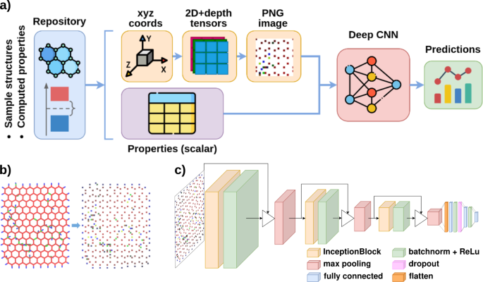
The general features of the framework used for the construction of the dataset and the subsequent training and testing of the neural networks is illustrated in Fig. 1a.

(a) Scheme of the GrapheNet framework, plotted with drawio³⁸; (b) example of encoding a GO sample, rendered with VMD³⁹, into an image, generated with the proposed approach (see Methods) and plotted with OpenCV⁴⁰ and Pillow⁴¹; (c) architecture of the GrapheNet CNN, plotted with drawio³⁸.

Full size image

First, the framework extracts information on the atomistic structure of individual NG samples and corresponding computed physical properties from available repositories. The datasets used in this work were constructed starting from publicly available repositories containing computed data on GO³³(20,396 samples containing 191–1949 atoms) and DG³⁴ (562,217 samples containing 206–447 atoms) systems. These two datasets also allow us to test the performance of the GrapheNet architecture for property predictions of non-periodic (GO samples) and periodic (DG samples) systems. A module for uniforming data formats for atom coordinates (encoded in the standard XYZ format⁴²) and chemico-physical properties was integrated in the overall framework. The properties of each sample are computed at the DFTB and DFT level for the GO dataset and for the DG dataset, respectively. Computed properties include formation energy (DG and GO dataset), total electronic energy, electron affinity, ionization potential, electronegativity, and Fermi energy (GO dataset).

To test the capabilities of GrapheNet, we used a subset of the overall data available, constituted by 7000 samples for both GO and DG (from now on called “reference’ datasets). For each sample, we transformed the coordinate values (x, y, z) and the type of atom (t) of each row of the XYZ file into a NxNx3 (GO) or NxNx1 (DG) tensor as discussed in the methods section. This transformation maps spatial information separately for each atom type in GO samples. Subsequently, the tensor constructed for each sample was converted into an RGB (for GO, in which the three color channels map the three different atom types) or grayscale (for DG) PNG image. A crop function was first applied to PNG images to remove unnecessary regions, allowing us to reduce the overall storage size of the entire datasets. During training runs, a variable size padding of black pixels was applied to cropped PNGs, ensuring the same size for all images used in training. These operations were performed using standard image manipulation libraries^40,41. An example of the representation obtained for GO samples is shown in Fig. 1b. Similar examples for DGs are provided as Supporting Information in Fig. S1.

The GrapheNet framework is based on a custom Inception-Resnet CNN model⁴³. The structure of the GrapheNet network is shown in Fig. 1c (see also the Methods section), while the structure of a single InceptionBlock is shown in Supporting Information (see Fig. S2). Predictions of the GrapheNet framework were compared with two other similar architectures based on a Resnet18⁴⁴ and a custom generic CNN (see Methods). The comparison showed that the GrapheNet architecture is able to provide the best tradeoff between training time and prediction capabilities. A complete comparison between these models has been reported in the Supporting Information (Table S1). The model was trained by feeding a PNG image as the input and a float value as the target property, evaluating the loss by means of a RMSE function for the formation energy and a MSE function for all other targets. When dealing with formation energy values, the network was fed with an additional n-dimensional vector representing the stoichiometry of the system. This additional feature should facilitate the training process by compensating for the strong dependence of absolute formation energy value from the composition of samples (see Methods). Further implementation details are provided in the Methods section.

Performance of GrapheNet in predicting GO and DG properties

The mean absolute error (MAE) and the mean absolute percentage error (MAPE) of Graphenet, obtained on the GO and DG datasets are shown in Table 1. MAE and MAPE constitute standard metrics for regression tasks. Further error metrics are provided as Supporting Information in Table S2.

Results show a remarkable accuracy for all predicted targets, with MAPE values below 2%. Interestingly, this threshold is well below the typical accuracy of computational chemistry methods used to evaluate target properties (about 4% for thermodynamic properties)^45,46, thus pointing to the potential of GrapheNet as a valuable predictive tool for the study of nanomaterials. Moreover, the extremely fast inference times (about 1 ms on the reference hardware) with respect to standard quantum mechanics calculations highlight the possibility of using this approach for high-throughput screening of very large structural datasets. The GrapheNet overall accuracy in the prediction of the GO and DG properties for the reference datasets is shown in Fig. 2. The distributions of the residual errors are shown in the Supporting Information (see Fig. S3).

GrapheNet predictions for the: (a) ionization potential ((R^2=0.850)); (b) electron affinity ((R^2=0.768)); (c) electronegativity ((R^2=0.807)); (d) Fermi energy ((R^2=0.928)); and (e) formation energy per atom for the GO reference dataset ((R^2=0.999)) and (f) formation energy per atom for the DG reference dataset ((R^2=0.993)).

Full size image

To assess the dependence of prediction accuracy on the size of the datasets, two further sets of simulations were performed. Reduced datasets for GO and DG models were generated by randomly picking 1/4 of the samples of the reference dataset (1750 images). A different augmented dataset was also generated, by applying image augmentation techniques. To this end, we applied three-fold rotation operations by multiples of (hbox {90}^circ) to the reduced dataset images, thus leaving the overall number of samples (7000) unchanged with respect to the reference dataset. Upon application of this data augmentation protocol, we obtained three additional images for each nanographene sample. These images represent the structure of the original sample rotated by (hbox {90}^circ), (hbox {180}^circ) and (hbox {270}^circ), respectively, and are fed to the network along with the corresponding physical properties (see Supporting Information, Fig. S4). The analysis of GrapheNet in relation to data augmentation techniques allows us to assess the prediction capabilities of the framework with a limited number of samples in the dataset. Moreover, as we lose the canonical orientation of images (see Methods) in the training dataset, data augmentation allows also us to assess the robustness of the framework in terms of rotational equivariance for 90-degrees rotations. As shown in Table 1, the behavior of GrapheNet reflects the variation in predictions accuracy expected as a function of the dataset size. In particular, data augmentation leads to prediction errors that are very close to those of the reference dataset. Moreover, it must be noted that image augmentation techniques greatly reduce the number of unique samples required for training the model. Hence, image augmentation constitutes an effective strategy for mitigating the overall computational burden associated with evaluating samples properties in large molecular systems and nanostructures.

To assess the dependence of the proposed encoding on the explicit representation of atom types, we retrained GrapheNet for the GO reference dataset using a single channel (grayscale) for all atom types. Interestingly, the prediction errors obtained in this case are only slightly larger (MAPE below 2.0% for all target properties; see Supporting Information, Table S3) than those obtained in the case of a full encoding of atom types through color channels. Therefore, mapping the position of atoms onto images implicitly encodes portions of information related to atom types, such as bond lengths. Indeed, relative atom positions can be associated to interatomic bonding patterns, which, in turn, depend on atom types.

From the computational point of view, GrapheNet shows in general comparable predictive performances with respect to state-of-the-art ML and deep learning frameworks for the prediction of molecular properties based on standard atomistic representations, such as the Coulomb matrix. However, GrapheNet demonstrates remarkable scalability with system size, considering the overall computing time required for both dataset generation and training, highlighting the potential of this approach for handling large systems. To evaluate numerically the performances of GrapheNet, and in particular of the image-based representation proposed, as a function of the system size to study the scalability, we partitioned the GO datasets in clusters with varying number of atoms, selected within the completed distribution (see Supporting Information, Fig. S5). In particular, we considered two sub-datasets of samples composed by 310–350 atoms, and 610–660 atoms, respectively. We then performed two sets of training and prediction runs, by using image-based and Coulomb matrix representations, fed in the same network architecture shown in Fig. 1c. More details on the implementation of Coulomb matrices are provided in the Methods section. This approach allows us to compare the effect of the encoding strategy on the overall computational load. For smaller-size samples, the Coulomb matrix representation leads to a slightly higher accuracy with respect to image representation (see Table S4 in the Supporting Information). However, the training time is significantly longer than that required by image encoding. For larger samples, however, the image representation proposed significantly outperforms the Coulomb matrix representation (Table S5 in the Supporting Information), with a significant decrease (by a factor of about 9 times) of the computing time required in the steps related to both encoding and training. The effect is even more evident when considering a larger datasets, with samples constituted by 310–660 atoms, where the image representation leads to an overall computing time that is 17 times smaller than that required by the Coulomb matrix representation (Table S6 in the Supporting Information). The striking computational performance of the image representation, which is at the core of GraphenNet, can mainly be ascribed to the efficiency of libraries for image encoding. In contrast, matrix representations of molecular structures can suffer from a O(2) scaling, which can constitute a significant limitation in the case of large systems such as nanographenes or nanostructures in general. It is also worth pointing out that, compared to Coulomb matrices, image representations introduce a quantization error, due to conversion from real values of 3D coordinates to integer values of pixel positions. Although deep neural networks (DNNs) could in principle be used in conjunction with flattened Coulomb matrix representations⁴⁷, this approach becomes quickly unfeasible in the case of large systems. In previous work, this approach has been applied to small systems, such as those in the QM9 dataset^48,49, containing molecules constituted by a maximum of 30 atoms. For larger systems, the memory scaling becomes a significant computational bottleneck. For a dataset of samples containing up to 660 atoms each, GrapheNet uses 15.7M parameters and 1.2M for the for the Coulomb matrices and image representation, respectively. In contrast, a DNN with 3 layers uses (sim ,,500)M parameters for samples composed by up to 350 atoms and a few billion parameters for samples composed by up to 660 atoms.

We also compared our approach with a representation based on the eigenvalues of the Coulomb matrix⁴⁷ to reduce the dimensionality of the problem. Using Coulomb matrix eigenvalues with classical regression methods, such as Kernel Ridge Regression (KRR)⁵⁰ and XGBoost⁵¹ leads to an accuracy that is comparable with that of a DNN, but to significantly shorter training times (see Table S7 in the Supporting Information). However, the computational complexity related to the evaluation of the eigenvalues leads to an overall lower performance with respect to the proposed image representation approach. We also considered a sub-set of large-sized samples, constituted by 1000–2000 atoms, to investigate the performance of our approach in dealing with large systems. It must be noted, for the sake of making a fair comparison between different methods and representations, that the Coulomb matrix representation was not investigated in this case, due to GPU memory limitations (which makes it another advantage of our method over workflows based on the Coulomb matrix). The prediction accuracy of GrapheNet is comparable to regression models and DNNs using eigenvalue representations (see Table S8 in the Supporting Information). However, the overall time required for building and training the models is significantly smaller for Graphenet, as a result of a much shorter computational load required for the generation of the representations. Additionally, the regressor models considered do not support batching, thus limiting the possibility of handling very large datasets.

Furthermore, we compared GrapheNet with a state-of-the-art materials graph neural network: M3GNet⁵², a framework based on graph neural networks designed for predicting material properties at the atomistic level. Both the model and the graph generation procedure are already implemented in the Materials Graph Library (MatGL)⁵³. We adopted the same implementation procedure used for GrapheNet (see Methods), with default parameters both for the model structure and for the graph generation procedure, and a cutoff distance set to 4Å. The comparison between GrapheNet and M3GNet on the GO reference dataset (see Table S9 in the Supporting Information), shows a slightly better accuracy prediction for M3GNet, but at the expense of a much larger computing time (about 74 times with respect to GrapheNet on the reference architecture) required for training. Indeed, while graphs are particularly well-suited for capturing complex local interactions and topological features at the atomic level, they constitute a computationally inefficient representation for large scale structures, such as those considered.

The relationship between computed accuracy and the distribution of features and targets in the datasets considered was further investigated to assess the performance of GrapheNet. As shown in Fig. 2a–d, the accuracy of models across the respective prediction ranges for GO samples can largely be ascribed to the peculiar multimodal distribution of targets, which are commonly treated with clustering techniques^54,55. Essentially, prediction errors are generally larger for target values corresponding to less sampled regions of the dataset, as expected. In turn, the multimodal distribution of targets observed can be related to the methodology used to build GO samples in the dataset, resulting in recurring structural patterns. The bias of the clustered distribution of structures of the initial dataset is also evident from the distribution of formation energy per atom for GO and DG samples (Fig. 2e, f), which is largely dependent on composition (see Supporting Information, Fig. S6). However, GrapheNet predictions of formation energy per atom are extremely accurate across the whole range of samples, including very large systems for the GO case (lower energy values in Fig. 2e). This behavior can be ascribed to the functional dependence of the computed loss on the stoichiometry of the system (see Methods) and to the peculiar distribution of structures in the samples. Interestingly, the prediction accuracy of GrapheNet improves significantly when the distribution of sample structures in the dataset considered is taken into account. To support this observation, we performed a nonlinear dimensionality reduction of a large set of spatially-invariant geometrical features for the GO dataset³³ by applying the uniform manifold approximation and projection (UMAP) method⁵⁶. Reduction of the GO feature space to two dimensions led to the occurrence of distinct clusters (see Fig. 3a). Remarkably, the overall number of clusters identified by DBSCAN⁵⁷ applied to the UMAP embedding (25 clusters) is the same value found by Motevalli et al.⁵⁸ by applying ILS⁵⁹, thus highlighting the potential of the UMAP method in the dimensionality reduction of complex spaces in the framework of materials representation. By re-training separately the GrapheNet network on portions of the original GO complete dataset selected on the basis of the UMAP clustering, which in some case leads to essentially unimodal distribution of targets, prediction errors lowered significantly. In particular, we selected three representative clusters with a mostly unimodal distribution of EA and IP and containing more than 500 samples (Fig. 3a). Prediction results for the retrained GrapheNet framework on each cluster are shown in Fig. 3b, c. The distribution of EA and IP within the selected clusters is shown in the Supporting Information (Fig. S7).

(a) Plot of the 2-dimensional UMAP dimensional reduction and color-coded clustering of samples as resulting from the application of the DBSCAN algorithm and selection of three representative clusters; (b) EA and (c) IP fits of GrapheNet retrained on data extracted from individual clusters, highlighted in purple, dark orange and green, respectively; (d–f) Samples of feature maps for low-level layers (layer 1, convolution 16, filter 5) of the GrapheNet network for selected GO samples with triangular (left), square (middle) and hexagonal (right) geometry.

Full size image

A feature map analysis was performed across the convolution layers of GrapheNet to highlight the relative relevance of input features and possible hierarchies. Inspection of feature maps revealed mainly patterns related to local structural properties, corresponding to low-level features (see for example Fig. 3d–f). The predictive performance of the network therefore suggests that, despite the lack of a clear localization of regions of interest related to target properties, the network is able to capture correlations with overall structural high-level features. This observation matches with the generally non trivial relationship between the topology of atoms and the spatial distribution of properties correlated to the electronic structure of NG flakes (for example, the topology of the HOMO and LUMO orbitals, which are—to a first approximation—related to the ionization potential and electron affinity, respectively. More details can be found in the Supporting Information, Fig. S8). The complex relationship between the structure of NG samples and resulting electronic properties (for example, topology of the molecular orbitals, etc.) is also evidenced by the lack of correlation with individual structural features (see Supporting Information, Fig. S9). As evidenced in previous work⁵⁸, a quantitative correlation between structure and electronic properties of NG samples requires a very large number of geometrical descriptors. In accordance with that, the significant predictive power of GrapheNet can therefore be related to the crucial role of high-level features in the CNN architecture, which essentially connect local properties.

This work unravels the potential of using images for encoding the structure of quasi-2D nanosystems and their application to CNNs for structure-property predictions. The approach outlined in this work highlights the computational and technical advantages of extending consolidated set of tools in computer vision and object detection to the representation of molecular systems and nanostructures. Unlike other methods based on the indirect encoding of the structural information of molecules into image-like representations^3,32, our approach attempts a direct mapping of the atom types and positions onto the three-dimensional tensor (2D pixel matrix and color channel) commonly used to encode images. Although limited to the representation of systems in which most of the structural information is conserved upon projection of atom positions onto a plane (which is exact for purely two-dimensional systems), this approach outlines the promising role of image analysis technologies for materials design and development. The quantitative evaluation of the predictive capabilities of the GrapheNet framework supports the use of images as an extremely flexible and efficient way to represent quasi-2D structures, such as nanographenes. In analogy with other methods for image analysis^60,61,62, this strategy leads to a less critical dependence of the numerical and predictive performances on the size of the system, as in traditional atom-based encodings. The numerical test performed in our work show the general suitability of CNN architectures to learn the relationship between complex local and non-local structural features and topologies and the resulting properties, as shown by the similar performance of different CNNs. Moreover, the proposed approach exhibit significant computational scaling properties and stability of prediction errors as a function of the system size, up to systems constituted by thousands of atoms (see Fig. S10 in the Supporting Information), thus suggesting remarkable potential in handling nanoscale materials. The generalizability of the proposed approach on other types of nanomaterials, and in particular, on more three-dimensional structures, was assessed by training GrapheNet on a dataset composed by defected phosphorene samples (DP)⁶³. Results (see Fig. S11 in the Supporting Information) show that GrapheNet is able to accurately predict the total energy per atom of defected phosphorene samples. Therefore, GrapheNet can in principle be generalized also to structures that are less planar than nanographenes. More details about the phosphorene dataset used and prediction results are discussed in the Methods section. In addition, the approach outlined in this work can possibly be extended to other systems requiring more complex encodings (higher-rank tensors). Work is in progress to extend the GrapheNet approach to the case of nanostructures with a more complex three-dimensional morphology and a larger number of atom types, by using higher-ranked tensors.

Potential applications and future work

One of the primary applications of GrapheNet lies in the accelerated discovery and design of new graphene-based materials. This is particularly relevant for example in the context of designing graphene metasurfaces, which can control electronic waves for applications in quantum computing and photonics⁶⁴. GrapheNet can also significantly impact the field of nanotechnology, especially in the fabrication of graphene nanostructures. The predictive accuracy of GrapheNet can facilitate the design and identification of optimal structures and functionalization patterns for the development of nanoscale devices, such as transistors and sensors. GrapheNet also holds significant potential for applications, for example as a screening tool to assess specific properties related to industrial requirements, thereby facilitating the commercial viability of nanographenes and the integration of data-centric digital technologies into existing manufacturing workflows. To this end, future work could also consider the development of interfaces and tools for users and workflow integration. The GrapheNet framework can also possibly be extended to predict the properties of other materials or systems composed by more than three atom types. This extension can be implemented for example by using 3D tensors from atom coordinates and by directly store them, thus skipping the conversion to images. An approach based on tensors would eliminate the constraint on dimensionality of image representations based on RGB channels. However, this approach would also lead to representations that are more difficult to interpret and analyse in terms of links between representations and corresponding chemico-physical properties. An alternative approach involves generating a separate grayscale image for each distinct atom type, encoding positions of atoms associated with that type, and using images as a “channels” stacked in a tensor. Although more complex, this approach could lead to a better interpretability of the representations. Moreover, the approach developed for GrapheNet can in principle be extended to the prediction of properties of 3D materials. As show in previous work,^65,66, voxels can for example be used to represent 3D entities as entries of a 3D grid. However, this approach may involve high computational costs and scalability issues for the representation of nanostructures composed by hundreds of atoms. Another possibility is to project the structure into three orthogonal planes, transform projections into images, and use these three images representation to train a multi-input version of the proposed Inception-Resnet model. This method of representing 3D objects is commonly used in technical drawing and engineering design, known as orthographic projection⁶⁷.

Dataset preparation

The datasets used in this work were based on the dataset discussed in³³ for GO and³⁴ for DG, respectively. The GO dataset consists of 20396 unique structures of finite-size GO nanoflakes and corresponding electronic properties evaluated at the DFTB level. The DG dataset consists of 562217 unique structures of periodic defective graphene sheets and corresponding electronic energy evaluated at the DFT level. For this latter case, the 2D periodicity is the same in all samples. For the GO dataset, the formation energy has been computed from the total electronic energy and from the individual energies of carbon, hydrogen and oxygen, using the DFTB+⁶⁸ package. From the original GO dataset, samples with non-physical values (i.e. NaN values) or with one or more target values equal to zero where also dropped. We also observed that the total energy of GO samples is strongly dependent on the local distribution of oxygen atoms on the surface of the flake (see Supporting Information, Fig. S12). To avoid the excessive burden of unrealistic high-energy configurations, GO samples with a mean distribution of oxygen-oxygen distances below the 20% of the overall mean (i.e., averaging over all samples in the dataset) were also dropped from the dataset. The GO dataset used in this work was built by randomly picking 7000 samples fulfilling these conditions. Similarly, 7000 samples were picked from the initial DG dataset, without any restriction. The 7000 element datasets for GO and DG, respectively, constitute the “reference” datasets discussed in the text. To assess the significance and relevance of both the reference and the complete initial datasets, the minimum, maximum, mean and standard deviation values for each target in the datasets is shown in the Supporting Information (see Table S10 and Table S11). Also, the comparison between the distributions of each target of the reference DG and GO datasets with respect their correspondent complete initial dataset is shown in the Supporting Information (see Fig. S13). The same clean-up procedure was applied to sub-datasets used for comparisons with Coulomb matrix and eigenvalues representations. For the UMAP analysis, only values whose targets were zero or NaN were removed from the initial dataset.

Regarding the DP dataset⁶³, it consist of 5342 unique pristine monolayer phosphorene structures as well as structures with monovacancies and divacancies containing 138–191 atoms, along with corresponding total energy properties evaluated at the DFT level. In this case, the entire dataset  has been used during the training process and its total energy per atom distribution is shown in the Supporting Information (see Fig. S14).

Image tensor representation

To ensure translational and rotational equivariance of the framework, coordinates of all samples are, when needed, transformed into a canonical representation. To this end, the coordinates of atoms are rotated so that the zigzag direction of the underlying graphene lattice aligns with the reference x axis and translated so that the atom with the minimum x and y coordinates is positioned at (0, 0). The (x, y, z) coordinates and the type t of atoms in each sample were transformed into tensors according to the following relationships:

Here, nint denotes the function that rounds to the nearest integer. The values (x_{min}), (y_{min}), (x_{max}), and (y_{max}) represent the minimum and maximum values of the x and y coordinates contained in the xyz file of the sample, respectively. Similarly, (Z_{min}) and (Z_{max}) indicate the minimum and maximum values of the z coordinate across the entire dataset. An empty (Ntimes Ntimes |{t}|) tensor is then filled so that the index of the cells is given by ((x_{matrix},y_{matrix},t)) (Eq. 1), while the indexed element contains the maximum normalized z value norm(z). Accordingly, the non-zero cells of the tensor represent atoms in the sample. The tensor is then multiplied cell-wise by 255 and casted to 8-bit unsigned integer in order to be compatible with an image-like representation. Lastly, the tensor is converted into image and cropped using standard image manipulation libraries^40,41. The cropping part is used to remove all the portions of the image that do not contain relevant information, that is, all the black pixels around the structure, in order to minimize the size of the images themselves. Through this representation, the combination of x and y coordinates is mapped as pixel positions on a 2D image, whereas the z coordinates determine the intensity of the corresponding pixels. In the presence of multiple atom types, as with the GO dataset, this contrast is depicted by utilizing distinct color channels in the image, employing RGB instead of grayscale, as with the DG dataset. The overall image generation workflow for both GO and DG datasets is described and deepened in the Supporting Information (see Figs. S15 and  S16).

Is worth mentioning that due to the fact that the size of the cropped image strictly depend on the size of the represented structure itself, and therefore for different structure sizes we can obtain different resolutions, a variable size padding of black pixels was applied during the training process in order to ensure the same size for all the images.

Coulomb matrix representation

According to Refs.^69,70, Coulomb matrices were computed as:

where (Z_i) represent the nuclear charge of the i-th atom while (R_i) represent its cartesian coordinates. The off-diagonal elements of the matrix represent the Coulombic repulsion between atoms i and j, whereas the diagonal elements capture a polynomial approximation of the atomic energies as a function of the nuclear charges, specifically (0.5Z_i^{2.4}). To speed up the calculation of matrices for large systems, Numba⁷¹ was used to compile the matrix generation function. Coulomb matrices were reordered by the norm of each row in decreasing order to create a unique and consistent representation of systems, which helps in reducing the variability due to the arbitrary ordering of atoms^69,70. A representation of the Coulomb matrix of a small GO sample is shown in the Supporting Information (see Fig. S17). To standardize Coulomb matrix dimensions for systems with varying number of atoms, each matrix was zero-padded to a uniform size equal to the maximum number of atoms within the dataset samples^69,70. Eigenvalues of Coulomb matrixes⁴⁷ were calculated as:

where M is the Coulomb matrix, (v_i) is the i-th column of the matrix and (lambda _i) is the i-th eigenvalue. Normalization was applied to both Coulomb matrix (man-mix scaler) and eigenvalues (max-min scaler or z-score for KRR) representations.

Network architecture

Numerical tests were performed by setting up predictive networks based on a custom CNN, a Resnet18 and a modified Inception-Resnet architecture. This latter constitutes the core of the GrapheNet framework. The Inception architecture leads generally to remarkable performances in tasks related to the analysis of images and enables a multi-level extraction of features within the same layer, through filters of different size. This capability enables the analysis of feature maps to identify potential correlations with the topology of properties related to the electronic structure of samples. The architecture of the GrapheNet CNN consists of three Inception blocks, each consisting of three convolutional layers, operating in parallel with different kernel sizes (1 (times) 1, 3 (times) 3 and 5 (times) 5). The outputs of the convolutional layers are concatenated and fed into the next layer. The convolutional blocks are similar to the ones used in the original Inception architecture⁴³, with the addition of residual connections, which bypass the convolutional layers and merge the input directly with the output. To ensure dimensional compatibility between the input and the output, a downsampling procedure is performed within the residual connection by a convolutional and batchnormalization layer. This approach allows the model to learn the residual function and make training deeper networks more feasible⁴⁴. This also helps to address the problem of vanishing gradients, which can occur in deep networks and make training difficult^72,73. Also, ReLU activation functions and batchnormalization layers were used to improve stability, accelerate convergence and reduce sensitivity to weight initialization. Lastly, the output of the last InceptionBlock is fed to a series of fully connected and dropout layers that performs the final prediction. Such dropout layer helps in the prevention of overfitting during the training of the network. The complete architecture, along with layers, dimensions and operations, of the Inception-Resnet model is shown in the Supporting Information (see Fig. S18). Resnet18⁴⁴ is a 18-layer network used as a standard benchmark in the context of CNNs for image analysis and classification. For this purpose, the original final layer of the network for predicting 1000 values with a softmax activation function was substituted with a sequence comprising a linear layer, followed by a ReLU activation function, a dropout layer, and a subsequent linear layer for predicting a single value. The custom CNN network developed for comparison purposes is composed by three blocks structured as consecutive convolutional and ReLu layers, with a batchnorm layer followed by a max pool layer between each block. Resulting feature maps are flattened and passed through two fully connected layers with batch normalization and ReLU activation. Finally, a dropout layer is applied to the output of the second fully connected layer, followed by a final fully connected layer that produces the output predictions. The scheme of the custom CNN network, and the detailed layers architecture are provided as Supporting Information (see Fig. S19 and S20). The DNN applied in the evaluation of models based on Coulomb eigenvalues representations was structured similarly to Ref.⁴⁷, and consists of three fully connected (linear) layers with ReLU activations after the first two layers. The network architecture includes an input layer, with a number of neurons depending on the number of Coulomb eigenvalues in the sample with the largest number of atoms within the dataset, a hidden layer with 140 neurons, and an output layer that performs the final prediction.

Targets and implementation

The CNN models were trained to predict the electronic properties of GO and DG samples using the values provided in the dataset as targets. For the prediction of formation energy (GO, DG) and total energy (DP) values, an additional vector representing the stoichiometry of the system was considered. This vector, along with the target value, was used to compute an RMSE loss function. In this case, the network is designed to produce a m-dimensional value as output, where (m=n+1) and n is the number of atom types (3 for GO, 1 for DG and DP). Accordingly, prediction of target properties p were computed as:

where (o_{i}) are the components of the m-dimensional output, (n_i) is the number of atoms of type i and Ntypes is the number of different atom types.

Models were implemented using the PyTorch Lightning framework⁷⁴. An assessment of the main hyperparameters (learning rate and the batch size) was performed. Namely, we tested the network by using the values of 0.001, 0.01 and 0.1 for the learning rate and 16, 32 and 64 for the batch size (see Supporting Information, Tables S12 and S13). Best results were obtained by using the Adam optimizer with a learning rate of 0.01 and a batch size of 32 for 150 epochs. Only for the M3GNet case, best results were obtained by using a learning rate of 0.001 instead of 0.01. Moreover, the ReduceLROnPlateau scheduler⁷⁵ was applied, which reduces the learning rate by a factor of 0.1 when the validation loss metric does not improve for 20 consecutive epochs. Is worth to mention that the ReduceLROnPlateau scheduler automatically adjusts the learning rate in response to stagnation in validation performance, reducing the need for manual learning rate fine-tuning by optimizing convergence, improving stability, and minimizing the risk of overshooting during training. An early stop callback was triggered if the validation loss metric stopped improving for 45 consecutive epochs which, combined with a callback to save the best model that minimizes validation loss, allows to mitigate overfitting. The optimized model is then used in the testing phase to perform the target predictions. Train and validation loss and accuracy for learning curves for the reference datasets (see Supporting Information, Figs. S21 and S22) show a good generalization to the validation data and no evident overfitting of the training data. All datasets used in numerical evaluations were split into fractions of 70% for training, 15% for validation and 15% for testing. Model training and predictions were performed on the SPRITZ computing cluster (CNR-ISMN Bologna, Italy) equipped with NVidia A40 GPUs. Computing times reported in this work refer to calculations performed on a single GPU. Training on multiple targets was performed in parallel on different computing nodes. Cross-validation was performed on the GO reference dataset to evaluate the variance and predictive accuracy of the proposed training/validation/test split with respect to k-folds, with 6 and then with 12 folds. Even without cross-validation, the proposed split shows comparable biases and comparable or slightly higher variances with respect to the cross-validation approach with 6 and 12 folds (see Supporting Information, Table S14). The DNN was also implemented using Pytorch Lightning and applying the same splitting used for GrapheNet. For XGBoost and KRR, the implementations are provided respectively by the XGBoost Python package⁵¹ and scikit-learn⁷⁶. For the XGBoost and KRR regression models, the training set was built by merging the training (70%) and validation (15%) sets  used for Graphenet, while the test set (15%) was unchanged.

The codes used to produce the results presented in this paper are available at https://github.com/daimoners/GrapheNet/tree/published. Future developments will be accessible in the main branch of the same repository (link: https://github.com/daimoners/GrapheNet/tree/master).

1. Cubuk, E. D., Malone, B. D., Onat, B., Waterland, A. & Kaxiras, E. Representations in neural network based empirical potentials. J. Chem. Phys. 147, 785. https://doi.org/10.1063/1.4990503 (2017).

   Article  CAS  Google Scholar 

2. Faber, F., Lindmaa, A., Von Lilienfeld, O. A. & Armiento, R. Crystal structure representations for machine learning models of formation energies. Int. J. Quant. Chem. 115, 1094–1101. https://doi.org/10.1002/qua.24917 (2015).

   Article  CAS  Google Scholar 

3. Wilkinson, M. R., Martinez-Hernandez, U., Wilson, C. C. & Castro-Dominguez, B. Images of chemical structures as molecular representations for deep learning. J. Mater. Res. 37, 2293–2303. https://doi.org/10.1557/s43578-022-00628-9 (2022).

   Article  ADS  CAS  Google Scholar 

4. Goswami, L., Deka, M. K. & Roy, M. Artificial intelligence in material engineering: A review on applications of artificial intelligence in material. Engineering. https://doi.org/10.1002/adem.202300104 (2023).

   Article  Google Scholar 

5. Axelrod, S. et al. Learning matter: Materials design with machine learning and atomistic simulations. Accounts Mater. Res. 3, 343–357. https://doi.org/10.1021/accountsmr.1c00238 (2022).

   Article  CAS  Google Scholar 

6. Rupp, M., Tkatchenko, A., Müller, K.-R. & von Lilienfeld, O. A. Fast and accurate modeling of molecular atomization energies with machine learning. Phys. Rev. Lett. 108, 58301. https://doi.org/10.1103/PhysRevLett.108.058301 (2012).

   Article  ADS  CAS  Google Scholar 

7. Hansen, K. et al. Machine learning predictions of molecular properties: Accurate many-body potentials and nonlocality in chemical space. J. Phys. Chem. Lett. 6, 2326–2331. https://doi.org/10.1021/acs.jpclett.5b00831 (2015).

   Article  CAS  PubMed  PubMed Central  Google Scholar 

8. Behler, J. & Parrinello, M. Generalized neural-network representation of high-dimensional potential-energy surfaces. Phys. Rev. Lett. 98, 146401. https://doi.org/10.1103/PhysRevLett.98.146401 (2007).

   Article  ADS  CAS  PubMed  Google Scholar 

9. De, S., Bartók, A. P., Csányi, G. & Ceriotti, M. Comparing molecules and solids across structural and alchemical space. Phys. Chem. Chem. Phys. 18, 13754–13769. https://doi.org/10.1039/c6cp00415f (2016).

   Article  CAS  PubMed  Google Scholar 

10. Pattanaik, L. & Coley, C. W. Molecular representation: Going long on fingerprints. Chem 6, 1204–1207. https://doi.org/10.1016/J.CHEMPR.2020.05.002 (2020).

    Article  CAS  Google Scholar 

11. Raghunathan, S. & Priyakumar, U. D. Molecular representations for machine learning applications in chemistry. https://doi.org/10.1002/qua.26870 (2022).

12. Weininger, D. SMILES, a chemical language and information system. 1. Introduction to methodology and encoding rules. J. Chem. Inf. Comput. Sci. 28, 31–36. https://doi.org/10.1021/ci00057a005 (2002).

    Article  Google Scholar 

13. Wigh, D. S., Goodman, J. M. & Lapkin, A. A. A review of molecular representation in the age of machine learning. https://doi.org/10.1002/wcms.1603 (2022).

14. Na, G. S., Chang, H. & Kim, H. W. Machine-guided representation for accurate graph-based molecular machine learning. Phys. Chem. Chem. Phys. 22, 18526–18535. https://doi.org/10.1039/D0CP02709J (2020).

    Article  PubMed  Google Scholar 

15. Fang, X. et al. Geometry-enhanced molecular representation learning for property prediction. Nat. Mach. Intell. 4, 127–134. https://doi.org/10.1038/s42256-021-00438-4 (2022).

    Article  Google Scholar 

16. Lorenzoni, A., Muccini, M. & Mercuri, F. Morphology and electronic properties of N, N’-Ditridecylperylene-3,4,9,10-tetracarboxylic diimide layered aggregates: From structural predictions to charge transport. J. Phys. Chem. C 121, 21857–21864. https://doi.org/10.1021/acs.jpcc.7b05365 (2017).

    Article  CAS  Google Scholar 

17. Baldoni, M. & Mercuri, F. Evidence of benzenoid domains in nanographenes. Phys. Chem. Chem. Phys. 17, 2088–2093. https://doi.org/10.1039/C4CP04848B (2015).

    Article  CAS  PubMed  Google Scholar 

18. Mercuri, F., Baldoni, M. & Sgamellotti, A. Towards nano-organic chemistry: Perspectives for a bottom-up approach to the synthesis of low-dimensional carbon nanostructures. Nanoscale 4, 369–379. https://doi.org/10.1039/C1NR11112D (2012).

    Article  ADS  CAS  PubMed  Google Scholar 

19. Selli, D. & Mercuri, F. Correlation between atomistic morphology and electron transport properties in defect-free and defected graphene nanoribbons: An interpretation through Clar sextet theory. Carbon 75, 190–200. https://doi.org/10.1016/j.carbon.2014.03.052 (2014).

    Article  CAS  Google Scholar 

20. Selli, D., Baldoni, M., Sgamellotti, A. & Mercuri, F. Redox-switchable devices based on functionalized graphene nanoribbons. Nanoscale 4, 1350. https://doi.org/10.1039/c2nr11743f (2012).

    Article  ADS  CAS  PubMed  Google Scholar 

21. Baldoni, M., Sgamellotti, A. & Mercuri, F. Electronic properties and stability of graphene nanoribbons: An interpretation based on Clar sextet theory. Chem. Phys. Lett. 464, 202–207. https://doi.org/10.1016/j.cplett.2008.09.018 (2008).

    Article  ADS  CAS  Google Scholar 

22. Silkin, V. M., Kogan, E. & Gumbs, G. Screening in graphene: Response to external static electric field and an image-potential problem. Nanomaterials 11, 789. https://doi.org/10.3390/NANO11061561 (2021).

    Article  Google Scholar 

23. Xu, F. et al. Computational screening of TMN4 based graphene-like BC6N for CO2 electroreduction to C1 hydrocarbon products. Mol. Catal. 530, 112571. https://doi.org/10.1016/J.MCAT.2022.112571 (2022).

    Article  CAS  Google Scholar 

24. Verma, A. M., Honkala, K. & Melander, M. M. Computational screening of doped graphene electrodes for alkaline CO2 reduction. Front. Energy Res. 8, 606742. https://doi.org/10.3389/fenrg.2020.606742 (2021).

    Article  Google Scholar 

25. Fernandez, M., Shi, H. & Barnard, A. S. Quantitative structure-property relationship modeling of electronic properties of graphene using atomic radial distribution function scores. J. Chem. Inf. Model. 55, 2500–2506. https://doi.org/10.1021/acs.jcim.5b00456 (2015).

    Article  CAS  PubMed  Google Scholar 

26. Fernandez, M., Shi, H. & Barnard, A. S. Geometrical features can predict electronic properties of graphene nanoflakes. Carbon 103, 142–150. https://doi.org/10.1016/j.carbon.2016.03.005 (2016).

    Article  CAS  Google Scholar 

27. Motevalli, B., Sun, B. & Barnard, A. S. Understanding and predicting the cause of defects in graphene oxide nanostructures using machine learning. J. Phys. Chem. C 124, 7404–7413. https://doi.org/10.1021/acs.jpcc.9b10615 (2020).

    Article  CAS  Google Scholar 

28. Dong, Y. et al. Bandgap prediction by deep learning in configurationally hybridized graphene and boron nitride. NPJ Comput. Mater. 5, 26. https://doi.org/10.1038/s41524-019-0165-4 (2019).

    Article  ADS  CAS  Google Scholar 

29. Yamawaki, M., Ohnishi, M., Ju, S. & Shiomi, J. Multifunctional structural design of graphene thermoelectrics by Bayesian optimization. Sci. Adv. 4, 74. https://doi.org/10.1126/sciadv.aar4192 (2018).

    Article  CAS  Google Scholar 

30. Wan, J., Jiang, J.-W. & Park, H. S. Machine learning-based design of porous graphene with low thermal conductivity. Carbon 157, 262–269. https://doi.org/10.1016/j.carbon.2019.10.037 (2020).

    Article  CAS  Google Scholar 

31. Yan, X. et al. In silico profiling nanoparticles: Predictive nanomodeling using universal nanodescriptors and various machine learning approaches. Nanoscale 11, 8352–8362. https://doi.org/10.1039/C9NR00844F (2019).

    Article  CAS  PubMed  Google Scholar 

32. Goh, G. B., Siegel, C., Vishnu, A., Hodas, N. O. & Baker, N. Chemception: A deep neural network with minimal chemistry knowledge matches the performance of expert-developed SAR/QSPR Models. ArXiv 1706.06689 (2017).

33. Barnard, A., Soumehsaraei, M., Benyamin, S. B. & Lai, L. Neutral graphene oxide data Set. v1. CSIRO. Data collection. https://doi.org/10.25919/5e30b44a7c948 (2019).

34. Kyle, M. & Isaac, T. Big Graphene Dataset. https://doi.org/10.4224/c8sc04578j.data (2019).

35. Elstner, M. et al. Self-consistent-charge density-functional tight-binding method for simulations of complex materials properties. Phys. Rev. B 58, 7260. https://doi.org/10.1103/PhysRevB.58.7260 (1998).

    Article  ADS  CAS  Google Scholar 

36. Kresse, G. & Furthmüller, J. Efficiency of ab-initio total energy calculations for metals and semiconductors using a plane-wave basis set. Comput. Mater. Sci. 6, 15–50. https://doi.org/10.1016/0927-0256(96)00008-0 (1996).

    Article  CAS  Google Scholar 

37. Hafner, J. Ab-initio simulations of materials using VASP: Density-functional theory and beyond. J. Comput. Chem. 29, 2044–2078. https://doi.org/10.1002/JCC.21057 (2008).

    Article  CAS  PubMed  Google Scholar 

38. JGraph. draw.io. https://github.com/jgraph/drawio (2021).

39. Humphrey, W., Dalke, A. & Schulten, K. VMD—visual molecular dynamics. J. Mol. Graph. 14, 33–38. https://doi.org/10.1016/0263-7855(96)00018-5 (1996).

    Article  CAS  PubMed  Google Scholar 

40. Bradski, G. The OpenCV Library. Dr. Dobb’s Journal of Software Tools. https://github.com/opencv/opencv (2000).

41. Murray, A. et al. Python-pillow/pillow: 10.4.0. https://doi.org/10.5281/zenodo.12606429 (2024).

42. Verstraelen, T. et al. IOData: A python library for reading, writing, and converting computational chemistry file formats and generating input files. J. Comput. Chem. 42, 458–464. https://doi.org/10.1002/JCC.26468 (2021).

    Article  CAS  PubMed  Google Scholar 

43. Szegedy, C. et al. Going deeper with convolutions. In Proceedings of the IEEE Computer Society Conference CVPR 1–9. https://doi.org/10.1109/CVPR.2015.7298594 (2015).

44. He, K., Zhang, X., Ren, S. & Sun, J. Deep residual learning for image recognition. In Proceedings of the IEEE Computer Society Conference CVPR 770–778. https://doi.org/10.1109/CVPR.2016.90 (2016).

45. Nicholls, A. Confidence limits, error bars and method comparison in molecular modeling. Part 1. The calculation of confidence intervals.. J. Comput. Aided Mol. Des. 28, 887–918. https://doi.org/10.1007/s10822-014-9753-z (2014).

    Article  ADS  CAS  PubMed  PubMed Central  Google Scholar 

46. Pernot, P. & Savin, A. Probabilistic performance estimators for computational chemistry methods: The empirical cumulative distribution function of absolute errors. J. Chem. Phys. 148, 241707. https://doi.org/10.1063/1.5016248 (2018).

    Article  ADS  CAS  PubMed  Google Scholar 

47. Hou, F. et al. Comparison study on the prediction of multiple molecular properties by various neural networks. J. Phys. Chem. A 122, 9128–9134. https://doi.org/10.1021/ACS.JPCA.8B09376 (2018).

    Article  CAS  PubMed  Google Scholar 

48. Ramakrishnan, R., Dral, P. O., Rupp, M. & Von Lilienfeld, O. A. Quantum chemistry structures and properties of 134 kilo molecules. Sci. Data 1, 1–7. https://doi.org/10.1038/sdata.2014.22 (2014).

    Article  CAS  Google Scholar 

49. Ruddigkeit, L., Van Deursen, R., Blum, L. C. & Reymond, J. L. Enumeration of 166 billion organic small molecules in the chemical universe database GDB-17. J. Chem. Inf. Model. 52, 2864–2875. https://doi.org/10.1021/CI300415D (2012).

    Article  CAS  PubMed  Google Scholar 

50. Vovk, V. Kernel ridge regression. Empirical Inference: Festschrift in Honor of Vladimir N. Vapnik 105–116. https://doi.org/10.1007/978-3-642-41136-6_11 (2013).

51. Chen, T. & Guestrin, C. XGBoost: A scalable tree boosting system. In Proceedings of the ACM SIGKDD International Conference on Knowledge Discovery and Data Mining 785–794. https://doi.org/10.1145/2939672.2939785 (2016).

52. Chen, C. & Ong, S. P. A universal graph deep learning interatomic potential for the periodic table. Nat. Comput. Sci. 2, 718–728. https://doi.org/10.1038/s43588-022-00349-3 (2022).

    Article  PubMed  Google Scholar 

53. Ko, T. W. et al. Materials Graph Library. https://doi.org/10.5281/zenodo.8025189 (2021).

54. Zhang, J., Lin, G., Li, W., Wu, L. & Zeng, L. An iterative local updating ensemble smoother for estimation and uncertainty assessment of hydrologic model parameters with multimodal distributions. Water Resour. Res. 54, 1716–1733. https://doi.org/10.1002/2017WR020906 (2018).

    Article  ADS  Google Scholar 

55. Yang, Q. et al. Multimodal estimation of distribution algorithms. IEEE Trans. Cybern. 47, 636–650. https://doi.org/10.1109/TCYB.2016.2523000 (2017).

    Article  Google Scholar 

56. McInnes, L., Healy, J. & Melville, J. Uniform Manifold approximation and projection for dimension reduction. ArXiv, UMAP (2018).

57. Ester, M., Kriegel, H.-P., Sander, J. & Xu, X. A density-based algorithm for discovering clusters in large spatial databases with noise. In KDD-96 226–231 (1996).

58. Motevalli, B., Parker, A. J., Sun, B. & Barnard, A. S. The representative structure of graphene oxide nanoflakes from machine learning. Nano Futures 3, 743. https://doi.org/10.1088/2399-1984/ab58ac (2019).

    Article  CAS  Google Scholar 

59. Parker, A. J. & Barnard, A. S. Selecting appropriate clustering methods for materials science applications of machine learning. Adv. Theory Simul. 2, 12. https://doi.org/10.1002/adts.201900145 (2019).

    Article  CAS  Google Scholar 

60. Si, Z., Zhou, D., Yang, J. & Lin, X. Review: 2D material property characterizations by machine-learning-assisted microscopies. Appl. Phys. A Mater. Sci. Process. 129, 1–13. https://doi.org/10.1007/S00339-023-06543-Y (2023).

    Article  ADS  Google Scholar 

61. Li, Y. et al. Rapid identification of two-dimensional materials via machine learning assisted optic microscopy. J. Materiomics 5, 413–421. https://doi.org/10.1016/J.JMAT.2019.03.003 (2019).

    Article  Google Scholar 

62. Masubuchi, S. et al. Deep-learning-based image segmentation integrated with optical microscopy for automatically searching for two-dimensional materials. NPJ 2D Mater. Appl. 4, 1–9. https://doi.org/10.1038/s41699-020-0137-z (2020).

    Article  Google Scholar 

63. Kývala, L., Angeletti, A., Franchini, C. & Dellago, C. Defected Phosphorene Dataset. https://doi.org/10.5281/zenodo.8421094 (2023).

64. Han, C.-D., Ye, L.-L., Lin, Z., Kovanis, V. & Lai, Y.-C. Deep-learning design of graphene metasurfaces for quantum control and Dirac electron holography. arXiv preprint arXiv:2405.05975 (2024).

65. Bougdid, Y. & Sekkat, Z. Voxels optimization in 3D laser nanoprinting. Sci. Rep. 10, 1–8. https://doi.org/10.1038/s41598-020-67184-2 (2020).

    Article  CAS  Google Scholar 

66. Pinheiro, P. O. et al. 3D molecule generation by denoising voxel grids. Adv. Neural. Inf. Process. Syst. 36, 347 (2023).

    Google Scholar 

67. French, T. E. & Vierck, C. J. The Fundamentals of Engineering Drawing and Graphic Technology (McGraw-Hill, 1978).

68. Hourahine, B. et al. DFTB+, a software package for efficient approximate density functional theory based atomistic simulations. J. Chem. Phys. 152, 124101. https://doi.org/10.1063/1.5143190 (2020).

    Article  ADS  CAS  PubMed  Google Scholar 

69. Himanen, L. et al. DScribe: Library of descriptors for machine learning in materials science. Comput. Phys. Commun. 247, 106949. https://doi.org/10.1016/J.CPC.2019.106949 (2020).

    Article  CAS  Google Scholar 

70. Li, S. et al. Encoding the atomic structure for machine learning in materials science. Wiley Interdiscipl. Rev. Comput. Mol. Sci. 12, 746. https://doi.org/10.1002/WCMS.1558 (2022).

    Article  Google Scholar 

71. Lam, S. K., Pitrou, A. & Seibert, S. Numba: A llvm-based python jit compiler. In Proceedings of the Second Workshop on the LLVM Compiler Infrastructure in HPC 1–6 (2015).

72. Hochreiter, S. The vanishing gradient problem during learning recurrent neural nets and problem solutions. Internat. J. Uncertain. Fuzziness Knowl.-Based Syst. 06, 107–116. https://doi.org/10.1142/S0218488598000094 (1998).

    Article  Google Scholar 

73. Roodschild, M., Gotay-Sardiñas, J. & Will, A. A new approach for the vanishing gradient problem on sigmoid activation. Progress Artif. Intell. 9, 351–360. https://doi.org/10.1007/s13748-020-00218-y (2020).

    Article  Google Scholar 

74. Falcon, W. The PyTorch lightning team. PyTorch Light. https://doi.org/10.5281/zenodo.3828935 (2019).

75. Al-Kababji, A., Bensaali, F. & Dakua, S. P. Scheduling techniques for liver segmentation: ReduceLRonPlateau vs OneCycleLR. In Communications in Computer and Information Science 1589 CCIS 204–212 (2022). https://doi.org/10.1007/978-3-031-08277-1_17.

76. Pedregosa, F. et al. Scikit-learn: Machine Learning in Python. J. Mach. Learn. Res. 12, 2825–2830 (2011).

    MathSciNet  Google Scholar 

Download references

Authors and Affiliations

1. DAIMON Lab, Istituto per lo Studio dei Materiali Nanostrutturati (ISMN), Consiglio Nazionale delle Ricerche (CNR), Via P. Gobetti 101, Bologna, 40129, Italy

   Tommaso Forni, Matteo Baldoni, Fabio Le Piane & Francesco Mercuri

2. Department of Control and Computer Engineering, Polytechnic University of Turin, Corso Castelfidardo 34/d, Turin, 10138, Italy

   Tommaso Forni

3. Department of Computer Science and Engineering, University of Bologna, via Zamboni 33, Bologna, 40126, Italy

   Fabio Le Piane

Contributions

F.M. conceived the approach and designed the framework and the experiments. T.F. carried out the implementations and performed the numerical experiments. F.L.P. contributed to the realization of numerical experiments. All authors analysed the results and reviewed the manuscript.

Corresponding author

Correspondence to Francesco Mercuri.

Competing interests

The authors declare no competing interests.

Publisher’s note

Springer Nature remains neutral with regard to jurisdictional claims in published maps and institutional affiliations.

Open Access This article is licensed under a Creative Commons Attribution-NonCommercial-NoDerivatives 4.0 International License, which permits any non-commercial use, sharing, distribution and reproduction in any medium or format, as long as you give appropriate credit to the original author(s) and the source, provide a link to the Creative Commons licence, and indicate if you modified the licensed material. You do not have permission under this licence to share adapted material derived from this article or parts of it. The images or other third party material in this article are included in the article’s Creative Commons licence, unless indicated otherwise in a credit line to the material. If material is not included in the article’s Creative Commons licence and your intended use is not permitted by statutory regulation or exceeds the permitted use, you will need to obtain permission directly from the copyright holder. To view a copy of this licence, visit http://creativecommons.org/licenses/by-nc-nd/4.0/.

Reprints and permissions