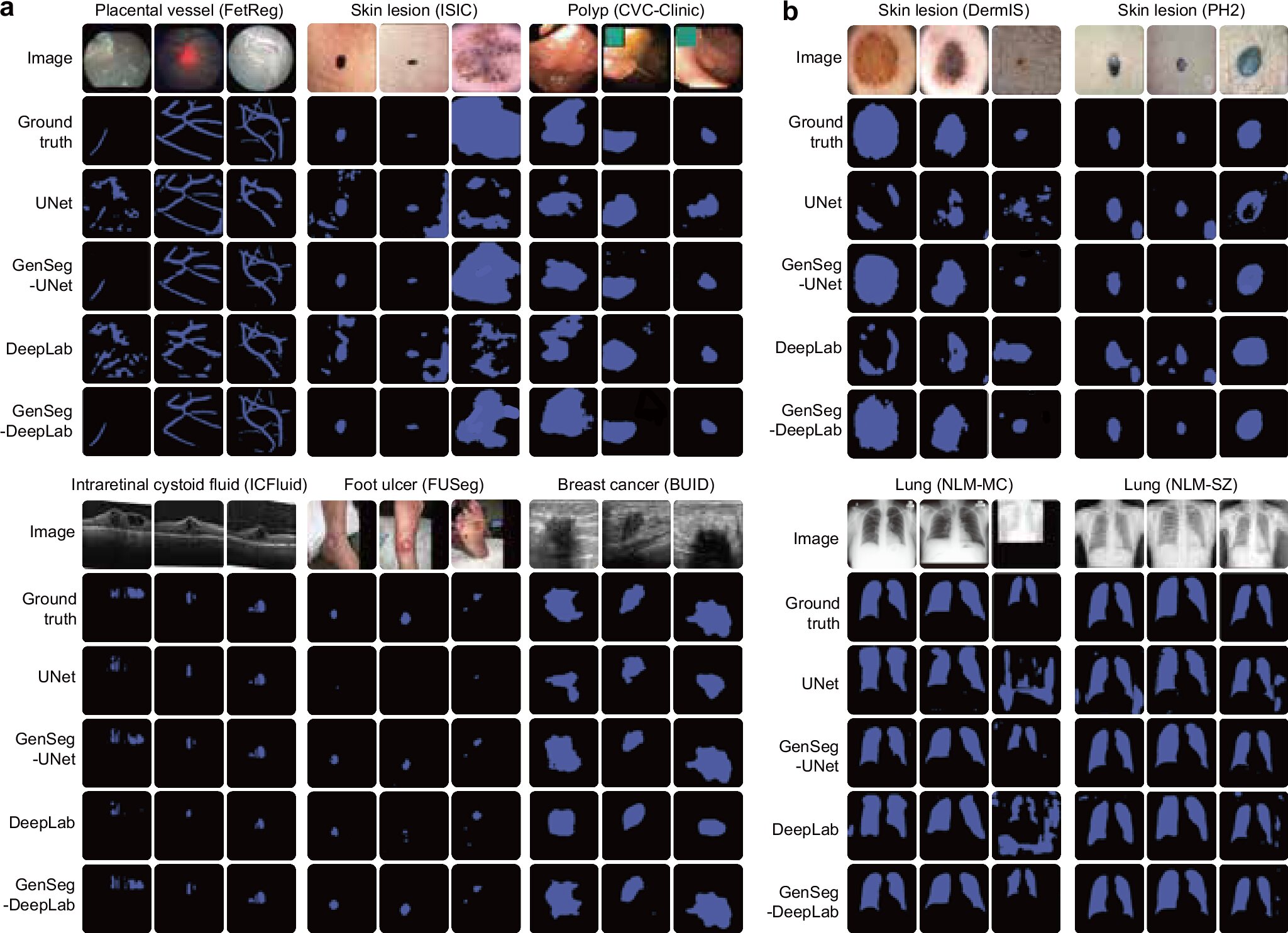
GenSeg improves in-domain and out-of-domain generalization performance across a variety of segmentation tasks covering diverse diseases, organs, and imaging modalities. Credit: Nature Communications (2025). DOI: 10.1038/s41467-025-61754-6 A new artificial intelligence (AI) tool could make it much easier—and cheaper—for doctors and researchers to train medical imaging software, even when only a small number of patient scans
Impact of agricultural industry transformation based on deep learning model evaluation and …
Introduction
The intensifying challenges of global climate change and the ongoing energy crisis have led countries worldwide to prioritize the transition to a low-carbon economy as a cornerstone of sustainable development. Agriculture, as a fundamental sector of production, plays a vital role in ensuring global economic stability and social well-being. However, it is also a significant source of greenhouse gas emissions. As such, facilitating the low-carbon transformation of agriculture has become essential for achieving sustainable development goals. China’s “dual carbon” strategy—targeting peak carbon emissions by 2030 and carbon neutrality by 2060—requires the agricultural sector to adopt more efficient and environmentally friendly production methods. Despite its importance, evaluating the effectiveness of agricultural transformation under this strategic framework remains a major challenge1,2. The dual carbon strategy, which emphasizes both emission reductions and increased carbon sequestration, represents a critical pathway to carbon neutrality3,4,5. Given agriculture’s substantial contribution to global greenhouse gas emissions, transforming this sector is crucial for meeting carbon reduction targets6. As the urgency of climate action intensifies, steering agriculture toward more sustainable and eco-friendly practices has become a global priority7,8. Meanwhile, deep learning—an advanced branch of machine learning—has demonstrated exceptional performance in fields such as image recognition and natural language processing. Its potential to enhance the evaluation of agricultural transformation is significant, offering improved accuracy and efficiency in capturing complex, multidimensional patterns within agricultural systems9,10,11.
However, current data-driven approaches to evaluating agricultural transformation face several limitations. Traditional models often neglect the spatiotemporal dynamics inherent in agricultural data, failing to account for evolving production patterns, climate variability, and soil conditions over time. Moreover, many existing models underutilize deep learning techniques, limiting their ability to model the intricate interdependencies among variables. These gaps highlight the pressing need for more advanced and effective evaluation frameworks capable of processing complex spatiotemporal data involved in agricultural transformation.
In the face of global climate change and energy crises, low-carbon transformation in agriculture has emerged as a crucial pathway toward achieving the “dual carbon” strategic goals. While numerous studies have explored the use of deep learning techniques to evaluate agricultural transformation, many existing approaches still exhibit significant limitations. For instance, Guo et al. (2024a) proposed a hybrid model integrating Convolutional Neural Network (CNN) and Long Short-Term Memory (LSTM) networks for climate prediction12. Although their model effectively captures spatiotemporal features, it lacks metaheuristic optimization and parameter tuning, limiting its ability to model the complex, dynamic interactions inherent in agricultural data. Consequently, its adaptability and stability in real-world agricultural scenarios remain inadequate. Moreover, prior research often focuses on single technologies or specific crop types, without adequately accounting for regional heterogeneity. Key factors such as climatic variation, soil characteristics, and policy interventions are frequently overlooked, resulting in poor generalizability across diverse agricultural contexts. To address these shortcomings, this study proposes a hybrid deep learning model that integrates CNN and LSTM architectures, optimized using the slime mould algorithm (SMA). SMA enhances the model’s ability to analyze spatiotemporal data by dynamically tuning hyperparameters, thereby improving performance in complex and heterogeneous environments. The CNN component efficiently extracts spatial features—such as planting density and irrigation infrastructure—using local receptive fields and parameter sharing. Simultaneously, the LSTM component captures long-term temporal dependencies by modeling time-series data, including meteorological variables (e.g., temperature, precipitation) and policy-driven changes, through gated recurrent units (GRUs). By combining CNN and LSTM and dynamically optimizing them with SMA, the proposed model overcomes the limitations of conventional spatiotemporal analysis frameworks. It significantly enhances adaptability to regional differences and dynamic environmental fluctuations. This approach not only establishes a robust evaluation framework for low-carbon agricultural transformation but also provides valuable methodological support for policymakers. It aids in optimizing resource allocation and advancing green agricultural development.
Additionally, this study aims to bridge gaps in traditional evaluation methods by introducing innovative solutions. Existing approaches often suffer from data collection challenges and inefficient evaluation processes13,14,15,16. By leveraging deep learning, this work proposes a more efficient, accurate, and scalable methodology for assessing agricultural transformation under the dual carbon framework.
The key innovations of this study are as follows. First, unlike Guo et al. (2024a), who utilized fixed hyperparameters, this study employed the SMA to dynamically optimize the hybrid CNN-LSTM architecture. SMA mimics the global search behavior of biological populations, helping to avoid local optima that often hinder traditional optimization methods when processing spatiotemporal data. This enhancement enables more effective analysis of multisource, heterogeneous agricultural data. Second, while previous studies have attempted to incorporate spatiotemporal features, few have systematically integrated satellite remote sensing, meteorological data, and field management information into a unified dynamic monitoring framework. This study addresses that gap by implementing a regionally adaptive adjustment strategy that accounts for geographic variability during model optimization, thereby improving cross-regional generalization. Third, given the high dimensionality and nonlinearity of agricultural transformation data, the proposed hybrid model not only performs hyperparameter tuning but also undergoes multiple independent experiments to validate its robustness. This approach offers a novel and reliable method for modeling complex agricultural systems. Collectively, these methodological advancements represent a significant improvement over the existing techniques. They establish a solid scientific foundation for precise evaluation and provide effective decision-support tools for promoting low-carbon agricultural transformation.
The remainder of this study is structured as follows: Sect. 1 introduces the study background, outlines key questions, identifies gaps in the existing literature, and presents the study’s structure. Section 2 reviews related work on agricultural transformation, deep learning models, and optimization algorithms. Section 3 details the methodology, including the development of the hybrid deep learning model and the implementation of the SMA. Section 4 presents the experimental design, dataset construction, and model performance evaluation. Section 5 discusses the implications of the findings, summarizes the study’s main contributions, and outlines potential applications and directions for future research.
Literature review
Since the Chinese government announced the “dual carbon” goals in 2020—targeting peak carbon emissions by 2030 and carbon neutrality by 2060—various industries have encountered both pressures and opportunities related to transformation and upgrading. The agricultural sector, as a traditionally high-energy-consuming industry, faces distinct challenges. Its transformation is essential not only for environmental protection but also for ensuring food security and promoting sustainable development17. Consequently, evaluating the outcomes of agricultural transformation has become a key area of interest for both researchers and policymakers.
In recent years, rapid advances in artificial intelligence (AI), particularly in deep learning, have significantly impacted the agricultural sector. These technologies have been widely applied in areas such as pest and disease identification and crop growth monitoring18,19. Such innovations have improved production efficiency while accelerating the transition toward low-carbon and intelligent agricultural practices. However, research focused on evaluating agricultural industry transformation using deep learning—especially within the framework of the dual carbon strategy—remains limited. For instance, Srivastava et al. (2022) developed a CNN-based model employing one-dimensional convolution operations to capture time-dependent relationships between environmental variables for winter wheat yield prediction. Their results showed the CNN outperformed other models in predictive accuracy20. Similarly, Saleem et al. (2022) applied various machine learning and deep learning algorithms in agricultural robotics, achieving notable performance gains21. Their findings revealed that deep learning-based models outperformed traditional methods, with RCNN reaching an 82.51% success rate in plant disease and pest detection. ResNet-18 and FCN also demonstrated superior performance in tasks such as crop-weed differentiation and land cover classification. Mohamed et al. (2023) provided a comprehensive review of trends in agricultural sustainability and technological innovation, highlighting emerging strategies such as precision farming, climate-smart techniques, and the integration of deep learning. They proposed innovative approaches to optimize crop yields, reduce ecological impact, and enhance global food security. These include quantum intelligence, meta-learning, deep reinforcement learning, curriculum learning, intelligent nanotechnology, blockchain technology, and CRISPR gene editing22. Cob-Parro et al. (2024) introduced an open-source infrastructure specifically optimized for developing and deploying AI-based models in agricultural environments23. In another study, Mujeeb and Javaid (2023) combined Spearman Correlation Analysis (SCA) and an improved shallow denoising autoencoder (ISDAE) with deep neural networks (DNNs), further enhanced by particle swarm optimization (PSO), to forecast carbon emissions in power systems24. Despite these technological advancements, several challenges persist in practical applications—particularly issues related to data acquisition and the limited generalizability of many deep learning models. Addressing these challenges remains critical to fully realizing the potential of AI in supporting agricultural transformation under the dual carbon framework.
Swarm intelligence metaheuristic algorithms—such as PSO, Genetic Algorithms (GA), and Ant Colony Optimization (ACO)—have attracted considerable attention for their effectiveness in optimizing deep learning and machine learning models. These algorithms simulate collective behaviors observed in nature, enabling them to efficiently search high-dimensional solution spaces while avoiding the local optima that often hinder traditional optimization methods. Their success has been particularly notable in tasks such as feature selection, model tuning, and parameter optimization for complex problems. Swarm intelligence algorithms have demonstrated unique advantages across various application domains. For example, they have been widely applied in optimizing machine learning models for tasks including cloud computing instance price prediction, early diagnosis of type 2 diabetes, and software defect detection. Salb et al. (2024) used an improved PSO algorithm to fine-tune multi-head deep learning models, significantly enhancing both prediction accuracy and model stability25. Similarly, Navazi et al. (2023) applied swarm intelligence algorithms to improve the accuracy and early-warning capabilities of diabetes diagnosis models26. In software defect detection, Petrovic et al. (2024) demonstrated that ACO effectively extracted key features from large-scale defect datasets, leading to improved predictive accuracy27. Zivkovic et al. (2023) employed swarm intelligence to optimize the Extreme Gradient Boosting (XGBoost) model and incorporated Shapley values to enhance feature interpretability, further boosting model performance28. In the realm of social media data analysis, Dobrojevic et al. (2024) used Genetic Algorithms (GAs) to optimize the XGBoost model, achieving substantial improvements in the detection of cyberbullying, gender discrimination, and harassment29. These studies collectively underscore the remarkable effectiveness of swarm intelligence metaheuristic algorithms in fine-tuning complex machine learning models, particularly in scenarios involving high-dimensional, nonlinear, and intricate datasets.
In the field of climate and environmental prediction, the application of deep learning models has become an emerging research focus. Guo et al. (2023) proposed a hybrid approach combining artificial neural networks (ANNs) with deep learning models to forecast monthly average and extreme temperatures in Zhengzhou30. By integrating the linear modeling capabilities of ANNs with the nonlinear feature extraction strength of models such as CNN, their study significantly improved prediction accuracy—particularly for extreme high-temperature events. However, the analysis was limited to a single city and did not involve multi-regional comparisons or the integration of dynamic spatiotemporal interactions. Expanding on this work, Guo et al. (2024a) explored the joint use of Deep Convolutional Neural Networks (DCNNs) and LSTM networks for monthly climate prediction. DCNNs were used to extract spatial features from climate data, while LSTM networks captured temporal dependencies. This hybrid model achieved high accuracy in predicting various climate indicators, including precipitation and wind speed. The experiments demonstrated lower prediction errors compared to traditional models under complex climate conditions. Nonetheless, the study did not incorporate optimization algorithms for hyperparameter tuning, which may limit the model’s adaptability in more dynamic scenarios.
For comparative performance analysis, Guo et al. (2024b) systematically evaluated DCNNs, LSTMs, GRUs, and Transformer models31. The findings showed that LSTM was most effective for modeling long-term dependencies, while Transformer excelled in capturing global correlations across climate variables. However, the absence of optimization strategies—such as metaheuristic algorithms—and inadequate handling of missing values during data preprocessing may have impacted the robustness of the results. In the context of air pollution prediction, He and Guo (2024) assessed the performance of LSTM, Recurrent Neural Networks (RNNs), and Transformer models in forecasting monthly PM2.5 concentrations in Dezhou32. LSTM achieved the lowest prediction errors due to its ability to model long-term dependencies in time series data, while the Transformer model was hindered by high computational complexity, limiting its practical application. The study also noted that nonlinear relationships between meteorological variables (e.g., wind speed and humidity) and pollutant concentrations remain a key modeling challenge. Further research by Guo, He, and Wang (2025) focused on ozone concentration prediction in Liaocheng, comparing the performance of LSTM and ANNs33. LSTM models showed better performance for daily ozone forecasts. However, their heavy reliance on real-time meteorological inputs reduced overall effectiveness. Additionally, the lack of multi-source data—such as satellite remote sensing—to enrich model inputs limited the ability to accurately predict sudden pollution events.
Recent advances in agricultural multisource data fusion and intelligent optimization have significantly expanded the application scope of deep learning and system modeling. For instance, Rokhva et al. (2024) developed an image recognition framework for the food industry using a pretrained MobileNetV2 model. Their lightweight network design enabled high-accuracy, real-time classification, and the proposed model compression strategies offer valuable insights for deploying agricultural remote sensing data in edge computing environments34. Building on this work, Rokhva and Teimourpour (2025) introduced a food classification model that integrated EfficientNetB7, the Convolutional Block Attention Module (CBAM), and transfer learning. Their use of attention mechanisms and data augmentation techniques presents effective solutions for aligning features in agricultural multimodal data, such as crop disease imagery and meteorological heat maps35. Additionally, Abbasi et al. (2025) applied circular economy principles to design a sustainable, closed-loop supply chain network. Their robust optimization framework addresses uncertainty and offers interdisciplinary support for dynamic resource allocation and policy resilience assessment in the context of agricultural low-carbon transitions36. While these studies span different domains, their contributions to lightweight model design, attention-based feature enhancement, and sustainable system optimization provide a strong interdisciplinary foundation for developing a multisource, data-driven evaluation model for agricultural transformation in this study.
Artificial intelligence and metaheuristic algorithms are increasingly applied across agriculture and environmental sciences, reflecting a growing multidisciplinary trend. For example, Gaber and Singla (2025) used Random Forest Regression (RFR) to predict groundwater distribution, with multivariate feature selection providing a data-driven framework for agricultural irrigation planning37. Similarly, El-Kenawy et al. (2024) introduced the Greylag Goose Optimization (GGO) algorithm, inspired by migratory bird behavior, offering novel swarm intelligence strategies for agricultural resource allocation38. In climate adaptation research, Alzakari et al. (2024) developed an enhanced CNN-LSTM model for early detection of potato diseases. Their multi-scale feature fusion effectively integrates local pathological features from leaf images with temporal disease progression patterns39. Elshabrawy (2025) reviewed waste management technologies for sustainable energy production, emphasizing the potential of hybrid metaheuristic algorithms—such as combinations of ACO and GAs—for agricultural waste recycling40. Regarding crop yield prediction, El-Kenawy et al. (2024) compared machine learning and deep learning approaches for forecasting potato yields. They found that integrating gradient boosting with Grey Wolf Optimization (GWO) substantially reduced errors caused by climate variability41. Despite these advances, most studies have yet to address spatiotemporal asynchrony in multisource agricultural data—including remote sensing, meteorological, and policy datasets—and often lack validation of cross-regional generalization. Furthermore, existing research on agricultural low-carbon transformation evaluation tends to focus on isolated technological pathways, rarely incorporating the dynamic effects of policy interventions. In contrast, this study proposes a hybrid CNN-LSTM model optimized by the SMA. SMA dynamically tunes model parameters, encoding regional climate adaptability as hyperparameter constraints. This approach enables the joint optimization of carbon footprint assessment and policy resilience. By overcoming the limitations of traditional methods in fusing cross-scale data and modeling nonlinear relationships, it provides an extensible evaluation framework to support the sustainable transformation of agricultural systems.
Table 1 summarizes the core methods, contributions, and limitations of representative studies on agricultural transformation evaluation. Existing research generally faces three key challenges. First, most models analyzing spatiotemporal features rely on fixed architectures and lack dynamic optimization. Second, metaheuristic algorithms are usually applied in isolation and are not fully integrated with deep learning models. Third, multisource data integration remains limited, hindering the ability to capture nonlinear interactions among climate, policy, and crop variables. In contrast, this study harnesses the global search capability of the SMA to coordinate CNN-LSTM spatiotemporal modeling. It also introduces region-specific feature weighting coefficients to enable a multidimensional, dynamic evaluation of agricultural transformation effects.
Full size table
Most existing studies have concentrated on case-specific applications involving individual technologies or crop types, often lacking systematic and comprehensive methodologies. Additionally, many have overlooked the impact of regional variability on agricultural transformation. To address these limitations, this study proposes an integrated evaluation framework that combines deep learning models—specifically CNN and LSTM networks—with the SMA, a swarm intelligence optimization technique. Unlike traditional methods, SMA excels at global search and is particularly effective for handling the spatiotemporal complexity of agricultural data, thereby enhancing the accuracy and stability of production forecasts. This study introduces three key innovations over conventional CNN-LSTM optimization frameworks: First, traditional models often rely on fixed hyperparameters and lack the flexibility to adapt to the dynamic nature of heterogeneous agricultural data. The proposed model overcomes this limitation by using SMA to automatically adjust critical hyperparameters—such as network architecture and learning rate—during training. This dynamic tuning enables the model to better adapt to complex agricultural features, significantly improving predictive accuracy and convergence speed. Second, unlike previous frameworks that depend on a single type of spatiotemporal data, the proposed model adopts a multi-channel input design. It simultaneously incorporates satellite remote sensing imagery, meteorological time series, and field management data. During the feature fusion stage, region-specific adaptive weighting factors are introduced to enhance the model’s sensitivity to geographic variability. This design improves generalizability across different agricultural regions—a common weakness in existing models. Third, validation experiments conducted across multiple agricultural subregions show that the proposed model maintains high predictive accuracy while exhibiting substantially lower error variance compared to traditional CNN-LSTM approaches. These results highlight its superior robustness and resilience to environmental and data-related disturbances. In summary, the CNN-LSTM-SMA model presents significant advancements in structural optimization, multisource data integration, and regional generalization. It offers a practical and adaptable framework for evaluating agricultural transformation and holds strong potential for supporting data-driven decision-making in low-carbon agricultural policy.
Key innovations include: (1) A deep learning framework that integrates diverse data sources—including satellite remote sensing, meteorological data, and field management information—to enable dynamic monitoring and evaluation of agricultural transformation. (2) Regionally adaptive model adjustment strategies that enhance predictive accuracy and generalization across varying geographic and climatic conditions.
Research methodology
This study proposes a hybrid model that integrates CNN, LSTM networks, and the SMA to enable a comprehensive, multidimensional, and dynamic evaluation of agricultural industry transformation outcomes. A core innovation of the model lies in the use of SMA for the dynamic optimization of CNN-LSTM hyperparameters. Additionally, the model incorporates a region-specific adaptive strategy to address the limitations of traditional methods in spatiotemporal data fusion and parameter tuning.
Construction of deep learning models: integrating CNN and LSTM
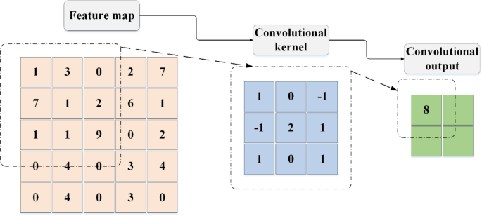
CNN is a type of deep learning architecture specifically designed for efficient image processing. They leverage several key features—local receptive fields, parameter sharing, and spatial hierarchies—to extract spatial features effectively. The basic structure of a CNN includes convolutional layers, activation functions, and pooling layers42,43,44. In the convolutional layer, the input data is processed through local receptive fields using filters (also known as convolution kernels) applied in a sliding-window manner. The convolution operation can be mathematically described by Eq. (1):
$$:left(f*gright)(i,j)=sum:_{m}sum:_{n}f(m,n)cdot:g(i-m,j-n)$$
(1)
In Eq. (1), (:f(m,n)) represents the input data, (:g(i-m,j-n)) denotes the weights of the convolution kernel, * indicates the convolution operation, and (:(i,:j)) represents the coordinates of the output feature map. This operation involves calculating the dot product of weights and input data, adding a bias term (:b), and introducing non-linearity through an activation function. The activation layer introduces non-linearity, enabling the model to learn and perform more complex tasks.
The process of the convolution operation is illustrated in Fig. 1.

Convolution operation process.
Full size image
The Pooling Layer, which consists of both Max Pooling and Average Pooling, aims to reduce the number of parameters, extract key features, and decrease sensitivity to the spatial location of the input data through downsampling45,46. The calculation for the Max Pooling operation is shown in Eq. (2):
$$:{P}_{max}(i,j)={max}_{m,nin:{Omega:}left(i,jright)}I(m,n)$$
(2)
In Eq. (2), (:{P}_{max}(i,j)) represents the pooled feature, (:I(m,n)) denotes the input feature map, and (:{Omega:}left(i,jright)) signifies the pooling window. The pooling operation process is illustrated in Fig. 2.

Process of Pooling Operation.
Full size image
The LSTM network is a specialized type of RNN designed to capture long-term dependencies in sequential data. It overcomes the vanishing gradient problem often encountered in traditional RNNs by incorporating a gating mechanism composed of input, output, and forget gates, along with a cell state featuring self-loops47,48,49. Table 2 outlines the key steps involved in processing input sequences within an LSTM network.
The model employs a CNN to extract spatial features from agricultural data, such as farmland distribution and soil types, using standard convolution operations. An LSTM network is then used to capture long-term dependencies in temporal variables, including meteorological trends and policy changes. The outputs of the CNN and LSTM are fused through a fully connected layer to generate a unified spatiotemporal feature representation. To improve the model’s adaptability to regional heterogeneity, a dynamic weight adjustment mechanism is introduced, as defined in Eq. (3):
Full size table
$$:{W}_{adapt}={upalpha:}cdot:{W}_{CNN}+(1-alpha:)cdot:{W}_{LSTM}$$
(3)
In Eq. (3), (:{upalpha:}) represents the regional feature weighting coefficient, which is dynamically optimized by the SMA based on the spatial distribution characteristics of the input data.
The pseudocode for the deep learning model training process is shown in Table 3.
Full size table
Parameter tuning and optimization of SMA
In this study, the fitness function plays a critical role in optimizing the model’s hyperparameters. A hybrid framework is proposed that integrates CNN, LSTM networks, and the SMA. The primary objective of this framework is to minimize the mean squared error (MSE) between the predicted outputs and the actual values. Given a multisource agricultural input dataset (:X) and its corresponding labels (:Y), the loss function is defined as shown in Eq. (4):
$$:mathcal{L}left({uptheta:}right)=frac{1}{N}sum:_{i=1}^{N}{({y}_{i}-{widehat{y}}_{i})}^{2}$$
(4)
In Eq. (4), N denotes the number of samples in the dataset, (:{y}_{i}) represents the true value of the i-th sample, and (:{widehat{y}}_{i}) is the corresponding predicted value. A lower MSE indicates higher prediction accuracy. Therefore, the objective of hyperparameter optimization is to minimize the MSE. During the optimization process, the SMA iteratively adjusts the model’s hyperparameters to reduce the MSE. After each iteration, SMA evaluates the current model configuration using the fitness function and determines whether further adjustments are necessary. As such, the fitness function plays a central role in guiding the optimization process.
SMA was selected as the optimization algorithm for this study due to its strong global search capabilities and adaptability. Inspired by the foraging behavior of slime molds, SMA simulates how these organisms adjust their movement based on odor concentration gradients. This behavior allows the algorithm to perform extensive searches in complex environments without requiring prior knowledge. Its robust global exploration makes it especially effective for high-dimensional, nonlinear optimization problems. Compared with other modern metaheuristic algorithms—such as the Crayfish Optimization Algorithm, Reptile Search Algorithm, and Red Fox Optimizer—SMA offers distinct advantages in addressing dynamically changing and complex tasks. While algorithms like the Crayfish Optimization Algorithm and Red Fox Optimizer may perform well in certain scenarios, SMA’s ability to avoid local optima through adaptive exploration results in more stable and accurate outcomes, particularly in tasks involving spatiotemporal data. It is important to note, however, that the selection of SMA does not imply it is universally superior. According to Wolpert’s “No Free Lunch Theorem,” no single optimization algorithm consistently outperforms others across all problem domains. SMA was chosen in this study based on its suitability for the specific challenges of modeling complex, spatiotemporal agricultural data. Its dynamic adjustment mechanism improved both convergence speed and optimization precision.
Advantages of SMA: Strong Global Search Capability: SMA mimics the foraging behavior of slime molds, enabling extensive exploration in high-dimensional spaces and effectively avoiding local optima. High Adaptability: The algorithm adapts well to diverse optimization tasks, making it particularly effective for handling the spatiotemporal complexity of agricultural data. High Optimization Efficiency: Compared with other optimization algorithms, SMA offers faster convergence and greater accuracy, especially during model training for complex agricultural datasets.
SMA is a bio-inspired optimization algorithm based on the foraging behavior of slime molds. It simulates the decision-making process these organisms use when locating food, optimizing model parameters in a similar fashion. During the search phase, slime molds rely on odor concentration cues to guide their movement toward food sources50,51,52. The mathematical formulation of this process is provided in Eq. (5) through (7).
$$:{X}_{t+1}={X}_{b}left(tright)+{v}_{b}cdot:left(text{W}cdot:{X}_{A}left(tright)-{X}_{B}left(tright)right),r
(5)
$$:{X}_{t+1}={v}_{c}cdot:text{X}left(tright),rge:p$$
(6)
$$:p=tanhleft|Sleft(iright)-{D}_{F}right|$$
(7)
In Eq. (5) to (7), (:{X}_{t+1}) represents the position vector of the slime mold population at time step t+1. (:{X}_{A}left(tright)) denotes the position vector of the food source at time step t, and (:{X}_{B}left(tright)) corresponds to the position vector of another individual in the slime mold population. W is the weight matrix, while (:{v}_{b}) and (:{v}_{c}) are velocity factors that control the movement speed of the slime molds. The variable r is a random number between 0 and 1, used to determine the movement strategy. The threshold p, calculated using Eq. (14), dictates whether the slime mold adopts a fast or slow movement strategy. (:Sleft(iright)) denotes the intensity or feature value of the i-th odor source, and (:{D}_{F}) is a predefined constant representing the food detection threshold53,54. The computation of the weight matrix W is detailed in Eq. (8) to (10).
$$:Wleft(SmellIndexleft(iright)right)=1+rcdot:text{lg}left(frac{{b}_{F}-Sleft(iright)}{{b}_{F}-{w}_{F}}+1right),condition$$
(8)
$$:Wleft(SmellIndexleft(iright)right)=1-rcdot:text{lg}left(frac{{b}_{F}-Sleft(iright)}{{b}_{F}-{w}_{F}}+1right),others$$
(9)
$$:SmellIndex=sortleft(Sright)$$
(10)
In Eq. (8) to (10), the variable (:SmellIndexleft(iright)) denotes the rank-based index of S, representing the intensity of odor sources or other features. (:{b}_{F}) and (:{w}_{F}) correspond to the boundary values of the food source and the slime mold’s current position, respectively. When the slime mold senses a high concentration of the food source, it increases the weight assigned to that area to enhance its ability to effectively encircle the food55,56. The weight adjustment process is detailed in Equations (11) to (13).
$$:{X}^{*}=text{r}text{a}text{n}text{d}cdot:left({U}_{B}-{L}_{B}right)+{L}_{B},rand
(11)
$$:{X}^{*}={X}_{b}left(tright)+{v}_{b}cdot:left(text{W}cdot:{X}_{A}left(tright)-{X}_{B}left(tright)right),r
(12)
$$:{X}^{*}={v}_{c}cdot:text{X}left(tright),rge:p$$
(13)
In Equations (11) to (13), (:{X}^{*}) represents the updated position of the slime mold individual. (:{L}_{B}) and (:{U}_{B}) define the lower and upper bounds of the slime mold’s position. (:z) is a random threshold used to determine the weight correction strategy57.
During this phase, the slime mold adjusts the width of its veins using propagating waves generated by biological oscillators, improving the efficiency of selecting optimal food sources. The oscillatory process is represented by the parameters (:W), (:{v}_{b}), and (:{v}_{c}), where the coordinated oscillation of (:{v}_{b}) and (:{v}_{c}) simulates the slime mold’s selective foraging behavior58,59.
To handle the nonlinear and high-dimensional nature of agricultural data, the SMA is employed for global hyperparameter optimization. While traditional SMA updates individual positions by simulating slime mold foraging behavior, this study enhances the weight update strategy by incorporating constraints specific to agricultural scenarios, as described in Eq. (14):
$$:{W}_{new}={W}_{old}+eta:cdot:{nabla:}_{region}({D}_{climate},{D}_{policy})$$
(14)
In Eq. (14), (:eta:) represents the learning rate, and (:{nabla:}_{region}) denotes the gradient constraint function derived from regional climate and policy data. This function encodes geographic differences as optimization directions, ensuring that hyperparameter selection aligns with the specific agricultural characteristics of each region. The optimization objective is to minimize the MSE, following the standard formulation.
For parameter tuning in deep learning models, SMA optimizes model weights by simulating the natural foraging behavior of slime molds. The parameter tuning and optimization process using SMA is illustrated in Fig. 3.

Parameter Tuning and Optimization Process of SMA.
Full size image
This study employs the SMA to optimize deep learning hyperparameters and enhance model performance. Specifically, SMA fine-tunes key parameters including the number of convolutional layers and kernel sizes in the CNN, the number of units in the LSTM, learning rate, optimizer choice, batch size, and the number of training epochs. The CNN’s structure—particularly its depth and kernel sizes—directly impacts its spatial feature extraction ability, while the number of LSTM units determines the capacity to capture temporal dependencies. Optimizer selection and learning rate are crucial for training efficiency, with appropriate learning rates enabling faster convergence. Batch size and training epochs also affect training speed and model accuracy. SMA optimizes these hyperparameters by simulating slime mold foraging behavior, effectively navigating the search space to avoid local optima issues common in grid or random search methods. This leads to faster convergence and improved generalization. The experiments integrate SMA within the deep learning framework to optimize the CNN and LSTM architectures’ key hyperparameters.
The SMA was used to optimize the hyperparameters of the deep learning models. The search ranges for these hyperparameters were determined based on practical application requirements, model performance, and insights from previous studies. For the CNN, the number of convolutional layers was set between 2 and 5 to avoid both overfitting from overly deep networks and underfitting from networks that are too shallow. Kernel sizes were chosen from [3 × 3,5 × 5,7 × 7], balancing feature extraction capability and computational efficiency. The stride was set to either 1 or 2; smaller strides improve feature detail, while larger strides speed up computation. Pooling window sizes were selected from [2 × 2,3 × 3], helping reduce computation and prevent overfitting. For the LSTM, the number of units was selected from [64,128,256], reflecting a trade-off between capturing long-term dependencies and computational cost. The learning rate was chosen from [0.0001,0.001,0.01] to ensure effective training without premature convergence. The Adam optimizer was used due to its strong performance and minimal need for parameter tuning. Batch size and training epochs were set to16,32,64 and [100,300,500], respectively. Batch size affects memory use and training stability, while epoch range balances learning completeness and overfitting risk. A summary of these search ranges is provided in Table 4.
Full size table
The pseudo code of SMA optimization process is shown in Table 5:
Full size table
To account for the inherent randomness of metaheuristic algorithms like SMA, multiple independent runs were conducted to ensure result reliability and stability. Each experiment was repeated 10 times with different initial conditions to reduce the risk of convergence to local optima. The average results from all runs provided a stable and representative measure of the optimization process, enhancing the robustness of the conclusions.
Figure 4 illustrates the architecture and operational flow of the proposed CNN-LSTM-SMA hybrid model. Multi-source agricultural data—including satellite remote sensing images, meteorological time series, and field management records—are fed into the CNN and LSTM modules via parallel channels. The CNN extracts spatial features such as farmland distribution and soil composition through convolutional operations, while the LSTM captures long-term temporal dependencies in variables like climate and policy interventions using GRUs. Outputs from both networks are fused through a weighted concatenation module, where the weights are dynamically optimized by the SMA. This optimization incorporates gradient constraints based on regional climate and policy heterogeneity. Through iterative updates, SMA adjusts critical hyperparameters—such as convolutional kernel sizes and the number of LSTM units—improving the model’s adaptability. Optimized parameters are continuously fed back into training. The fused spatiotemporal features then pass through a fully connected layer to produce an agricultural transformation effectiveness score, enabling comprehensive and dynamic evaluation. The schematic clearly depicts data flow, module interactions, and the feedback-driven optimization, highlighting the model’s innovative ability to integrate heterogeneous data and adapt to regional variability.

Structure and Optimization Process of the CNN-LSTM-SMA Hybrid Model.
Full size image
To enhance the model’s regional adaptability, a region-specific feature weighting coefficient (:{a}_{i}) is introduced during the CNN and LSTM feature fusion stage. This coefficient adjusts the contribution of features from different regions to the final prediction. The initial values of (:{a}_{i}) are derived by normalizing a prior indicator vector constructed from geographical attributes such as climate zones, soil types, and terrain relief, as shown in Eq. (15):
$$:{a}_{i}^{left(0right)}=frac{{x}_{i}}{sum:_{j=1}^{n}{x}_{j}}$$
(15)
where (:{x}_{i}) represents the feature intensity score of the i-th region, and n is the total number of regions. During model training, the SMA incorporates the regional weighting coefficients as tunable parameters within the individual encoding, alongside hyperparameters such as the number of CNN convolutional kernels and LSTM units. After each iteration, SMA evaluates the fitness of each individual based on prediction error—primarily using MSE—and fine-tunes the regional weights accordingly. The update strategy combines global exploration with local exploitation, enabling the model to dynamically adjust spatial feature weights based on the performance of input data from different regions. This mechanism significantly improves the model’s generalization and adaptability across regions.
Experimental design and performance evaluation
Datasets collection and experimental environment
This study collected multi-source data from 2000 to 2023, including agricultural production, meteorological conditions, soil properties, and crop growth cycles. The data were cleaned and normalized for input into the deep learning model. To capture temporal variations across multiple growing seasons, the dataset incorporates time series data spanning various scales. Additionally, agricultural field data from diverse geographic regions were included to enhance the model’s generalizability. An efficient experimental environment was established to develop and evaluate the hybrid deep learning models. The setup uses PyTorch 1.8.1 as the deep learning framework on a Windows Server 2010 operating system. Development was conducted in PyCharm Community Edition 2021.1, within a Python 3.7 environment managed by Anaconda 2021.5, alongside various scientific computing and data analysis libraries. For GPU acceleration, the system is equipped with a Tesla V100-32 GPU (32 GB memory) using the CUDA 10.2 architecture, enabling large-scale parallel computations and significantly improving training efficiency.
In multi-source data preprocessing, this study employs tailored workflows for remote sensing images, meteorological time series, and field management records. Remote sensing data undergo radiometric calibration, atmospheric correction, and resampling to a uniform spatial resolution of 10 m. Vegetation indices, such as Normalized Difference Vegetation Index (NDVI) and Enhanced Vegetation Index (EVI), are normalized to the [0, 1] range. Meteorological data are processed through timestamp-based interpolation to fill missing values and remove outliers, followed by z-score normalization (mean = 0, standard deviation = 1) to improve sensitivity to sudden weather changes. Field management data—such as planting density and fertilization frequency—are normalized using min-max scaling to ensure consistent input dimensions. Before model input, all data are organized into spatiotemporal samples via region-based sliding windows. Principal component analysis (PCA) is applied to remove redundant features, producing structurally consistent tensor inputs. This preprocessing pipeline enhances training stability and improves multi-source data fusion, providing a solid foundation for accurate predictions.
Parameters setting
Parameter settings are crucial in model training, directly influencing the model’s learning efficiency and generalization performance. This section details the key parameter configurations of the hybrid deep learning model used to evaluate agricultural industry transformation effects. These parameters have been carefully tuned to maximize prediction accuracy and robustness. The specific settings are summarized in Table 6.
Full size table
Performance evaluation
All figures and tables in this study are based on multi-source agricultural datasets from 2000 to 2023, including satellite remote sensing, meteorological time series, and field management records. They visually demonstrate the model’s ability to extract spatiotemporal features and perform dynamic optimization.
Application of hybrid deep learning models in evaluating the effects of agricultural industry transformation
Figure 5 illustrates how the hybrid deep learning models predict the impacts of agricultural industry transformation. These models achieve remarkable accuracy in forecasting crop yields, with an average precision exceeding 99%. The results show that the models effectively capture key factors influencing agricultural production, providing reliable yield predictions.

Evaluation of the Effects of Agricultural Industry Transformation Predicted by Hybrid Deep Learning Models.
Full size image
Figure 6 shows the evaluation of agricultural industry transformation effects across different regions using hybrid deep learning models. The deviation between the model’s predicted scores and the actual scores is minimal, with an average error of approximately 3.33%. This demonstrates the models’ effectiveness and reliability in assessing the impacts of agricultural transformation. Overall, the hybrid models exhibit high accuracy and stability, offering valuable support for decision-making in sustainable agriculture and providing scientific evidence to help achieve the dual carbon goals.

Evaluation of the Effects of Agricultural Industry Transformation in Different Regions by Hybrid Deep Learning Models.
Full size image
Comparison between model predictions and actual transformation effects
To comprehensively assess the performance of the SMA-optimized deep learning model, this study reports the fitness function scores recorded during training. Table 7 summarizes these fitness scores.
Full size table
The results show that the best fitness value of 0.987 indicates the model found solutions close to the optimum during training. The worst fitness value of 0.789 suggests that, although the model did not always reach peak performance in some epochs, it remained within an acceptable range. The mean fitness value of 0.899 and median of 0.902 demonstrate consistent performance and stability across multiple trials. The low standard deviation and variance further indicate a stable training process with minimal fluctuations, reflecting strong convergence. These statistics enable deeper analysis of the model’s performance over different training epochs. The rapid convergence and stable outcomes suggest the optimization process is effective. Future work will aim to further enhance the model’s performance.
To comprehensively evaluate the SMA-optimized deep learning model, a box plot of fitness function values across multiple independent runs is provided. Figure 7 illustrates the convergence behavior: Fig. 7(a) displays the median, interquartile range, and outliers from 50 independent runs, revealing the range and distribution of fitness values. Figure 7(b) reorganizes the numerical data for a detailed quantitative stability assessment. The results confirm that the model exhibits strong convergence and stability, with minimal fluctuations in fitness values across runs, demonstrating the robustness of the optimization algorithm.

Convergence analysis of the fitness function (a) Box plot; (b) Convergence performance.
Full size image
Figure 8 compares the model-predicted effects of agricultural industry transformation with the actual outcomes. The hybrid deep learning models demonstrate strong predictive performance for agricultural carbon emissions and carbon sequestration, with prediction errors consistently within 5%, indicating high accuracy.

Comparison between Model-Predicted Effects of Agricultural Industry Transformation and Actual Effects.
Full size image
Sensitivity analysis under different climate conditions and policy interventions
Figure 9 illustrates the stability of model predictions across different climate conditions. Under various climate scenarios, the average prediction error stays below 2.5%, with minimal standard deviations. This demonstrates the model’s strong adaptability to diverse climates and its ability to deliver stable, reliable predictions.

Prediction Stability of the Model under Different Climate Conditions.
Full size image
Table 8 presents a comparison of model performance along with statistical significance analysis. The proposed SMA-optimized model outperforms all other methods across key metrics, achieving an accuracy of 99.1%, a mean error of 2.11%, and a standard deviation of 1.12%. Compared to traditional regression models, it improves accuracy by 13.5% points (t = 6.32, p < 0.01) and reduces standard deviation by 2.12% points (t = 4.21, p < 0.01), demonstrating its strength in capturing complex nonlinear relationships and reducing prediction variability. Relative to DNNs, the proposed model requires 40 s more training time (220s vs. 180s) but gains 4.8% points in accuracy (t = 2.15, p < 0.05) and decreases standard deviation by 0.73% points (t = 1.87, p < 0.05), highlighting the effectiveness of SMA-based hyperparameter optimization in enhancing both precision and generalization. Although support vector machines (SVM) and decision trees train faster (120s vs. 220s), their predictive performance lags behind, with accuracy deficits of 7.0% and 10.9%, respectively, and nearly double the standard deviations. These findings underscore the importance of hybrid deep learning frameworks in effectively addressing the spatiotemporal heterogeneity inherent in agricultural systems. The statistical significance of all comparisons (p < 0.05) confirms the robustness and reliability of the proposed model, establishing it as a high-precision, adaptable tool for dynamic evaluation of low-carbon agricultural transformation.
Full size table
To provide a comprehensive evaluation of model performance, this study also includes Receiver Operating Characteristic (ROC) curves and inference time as supplementary metrics for classification tasks. Figure 10 compares the binary classification performance of various models in assessing agricultural transformation outcomes, while Table 9 summarizes the training and inference time efficiency of each model.

Performance Comparison of Different Models in Agricultural Transformation Classification Tasks.
Full size image
As shown in Fig. 10, the proposed model demonstrates superior classification performance with an Area Under the Curve (AUC) of 0.983. This high AUC indicates the model’s strong ability to accurately distinguish between different categories of agricultural transformation outcomes. The ROC curve further reveals that, at a threshold of 0.5, the model achieves an optimal balance between sensitivity (0.97) and specificity (0.98), reflecting robust discriminative power for both positive and negative classes. In contrast, the traditional regression model performs poorly (AUC = 0.812), largely because its linear assumptions limit its ability to capture nonlinear decision boundaries. Although the SVM improves classification through kernel-based transformations, its fixed kernel function is less effective at handling the multi-scale characteristics of agricultural data, resulting in a lower F1-score of 0.86.
Full size table
As shown in Table 9, the proposed SMA-optimized model requires slightly more total training time (220 s) than baseline models, notably the DNN, which completes training in 180 s. This increase is mainly due to the additional computational overhead of the SMA optimization loop. However, the model still achieves acceptable efficiency for real-time applications, with a per-batch training time of 79.8 milliseconds and an inference latency of 2.10 milliseconds per sample. Importantly, although the SMA’s global search mechanism adds overhead in early iterations, it effectively reduces the risk of getting trapped in local optima and decreases the total number of iterations required to reach optimal performance. This trade-off results in a balanced improvement in both predictive accuracy and computational efficiency.
Discussion
The hybrid deep learning model developed in this study—combining CNN and LSTM networks optimized with SMA—proved highly effective in evaluating agricultural industry transformation. It delivered both high prediction accuracy and stability, consistent with findings from related research. For example, Li et al. (2020) employed CNN to analyze satellite imagery for crop monitoring and yield estimation60. They demonstrated that CNN excel at capturing spatial information, thereby improving prediction accuracy. This supports our findings on the critical role of CNN in extracting spatial features from agricultural datasets. Similarly, Agyeman et al. (2022) used LSTM networks to forecast farmland irrigation demand, effectively handling time-series agricultural data based on meteorological and soil moisture records61. Their success reinforces the suitability of LSTMs for modeling temporal dependencies, further justifying the hybrid CNN-LSTM approach adopted here. Additionally, Xu et al. (2023) applied the SMA to optimize neural network weights and architectures for complex industrial data, enhancing model performance and generalization62. Although their domain differed, their results confirm the SMA’s capability to improve adaptability—aligning with this study’s goal of enhancing hybrid model sensitivity and expressiveness.
The proposed hybrid model offers notable advantages in assessing agricultural transformation effects. For instance, Liu et al. (2022) used a Transformer-based model for multi-source crop yield prediction, but its fixed-window attention limited spatial heterogeneity capture in small farmlands63. Moreover, without an optimization algorithm, their model showed high variability under extreme weather. In contrast, our study employs SMA to dynamically optimize convolution kernel sizes and LSTM units, boosting sensitivity to local features and abrupt changes. Likewise, Mokhtar et al. (2023) improved irrigation forecasting using an LSTM optimized with a GA, but their univariate temporal model could not address spatial variability in soil moisture64. The CNN-LSTM hybrid here overcomes this by fusing spatial and temporal features with weighted integration, substantially enhancing regional resource utilization assessment resolution.
Regarding regional adaptability, Bai et al. (2024) employed geographic information systems (GIS) and statistical models to evaluate policy effectiveness. However, their reliance on linear assumptions limited their ability to capture the nonlinear interactions among climate, crops, and policy variables65. In contrast, this study introduces dynamic weighting coefficients that incorporate regional climate zones and soil types into the feature weighting process. This enables the model to adaptively balance spatial and temporal feature contributions. For example, in drought-prone areas, the model increases the temporal weighting of meteorological data while simultaneously enhancing CNN-based extraction of spatial features related to irrigation infrastructure. This approach offers a more precise representation of water-saving policy impacts and provides interpretable decision support for designing region-specific policies.
In practical applications, the model’s dynamic optimization framework extends to areas such as agricultural carbon sink assessment and disaster risk forecasting. By integrating real-time satellite data, the model can dynamically update farmland carbon sink potential maps, aiding local governments in ecological compensation planning. In disaster warning scenarios, it combines short-term meteorological forecasts with historical disaster data to develop region-specific emergency response plans. Moreover, the model’s multi-source data fusion mechanism establishes a strong technical foundation for smart agriculture platforms and can be seamlessly integrated with agricultural Internet of Things (IoT) systems. This integration supports closed-loop management, spanning from data acquisition to decision feedback, ultimately accelerating the digital transformation of agriculture.
Overall, the study’s results align well with existing literature, and comparisons with prior research validate the proposed method’s reliability. These findings contribute to a deeper understanding of how hybrid deep learning models can be effectively applied in agricultural contexts.
Conclusion
Research contribution
This study presents a hybrid model that integrates deep learning with SMA optimization to predict the effects of agricultural industry transformation. Experimental results demonstrate that the proposed model significantly outperforms traditional regression models, decision trees, SVMs, and DNNs across key evaluation metrics—particularly in accuracy and stability. Training efficiency and consistency were further validated through fitness function scores and statistical analyses, including t-tests, confirming strong convergence and robust performance throughout the optimization process.
The CNN-LSTM-SMA hybrid model developed in this study offers a high-precision, adaptive tool for evaluating the impacts of agricultural transformation, with considerable practical value. Government agencies can use this model to dynamically assess regional carbon sequestration capacity and emission reduction efficiency, thereby informing targeted policy interventions. For instance, ecological compensation schemes could be refined using carbon footprint heatmaps generated by the model, while crop planting patterns could be adjusted based on climate adaptability projections. Agricultural technology companies may also embed the model into smart farming platforms to monitor real-time field data—such as soil moisture and weather variability—and dynamically optimize irrigation and fertilization practices, minimizing both resource waste and carbon emissions.
Additionally, the model has strong potential in disaster risk management. By integrating short-term extreme weather forecasts with historical disaster records, it can generate region-specific emergency response plans, helping decision-makers allocate mitigation resources more effectively. Future research should focus on integrating the model with agricultural IoT systems and developing edge computing solutions to support real-time, in-field inference. It is also essential to foster collaboration among policymakers, technology developers, and researchers to build a closed-loop system that seamlessly links data collection, model analysis, and decision-making. This interdisciplinary approach will accelerate the conversion of model outputs into actionable strategies. Through such integration and innovation, the proposed framework could serve as a core technological foundation for advancing global low-carbon agricultural transformation and supporting the achievement of carbon neutrality goals.
Future works and research limitations
Although the proposed model demonstrates strong performance, several limitations should be acknowledged. The study primarily relied on historical data for training and validation, which can be affected by issues such as poor quality, incompleteness, and time lag. Yet agricultural production is influenced by a complex set of dynamic factors—including climate variability, evolving policies, and fluctuating market conditions—that historical records may not fully capture. To improve adaptability, future research should consider integrating real-time data streams, enabling the model to better reflect current agricultural realities. Another key limitation involves regional variability. Agricultural practices, climate patterns, and soil characteristics differ significantly across geographic areas, which can affect model performance. For instance, the impacts of climate change on agriculture vary by location, potentially leading to higher prediction accuracy in some regions and reduced accuracy in others. This study did not fully address these regional disparities. Future work should explore methods for tailoring model parameters or incorporating localized data to enhance geographic generalizability. Incorporating real-time data also presents technical challenges, such as large-scale data transmission, data cleaning, and efficient processing. Building robust data pipelines and ensuring the accuracy and completeness of incoming data will be critical. The heterogeneity and uncertainty inherent in real-time sources add further complexity, particularly in managing missing or noisy data. Addressing these challenges should be a key priority for future research. Additionally, the model’s applicability across diverse agricultural systems requires further investigation. Variations in environmental conditions, policy frameworks, and farming practices may necessitate region-specific modeling approaches. Developing localized sub-models or integrating GIS with the SMA optimization framework could improve adaptability and performance across different contexts.
By addressing these limitations, future studies can enhance the robustness, accuracy, and applicability of the SMA-optimized deep learning model, thereby offering stronger decision-support tools for sustainable agricultural development.
Beyond technical considerations, the deployment of artificial intelligence (AI) models in agricultural settings introduces a range of ethical and socio-economic challenges. For example, if the training data is not sufficiently representative or contains regional biases, the resulting models may perform inconsistently across different populations or geographic areas, potentially leading to algorithmic bias. Such discrepancies can exacerbate regional disparities in agricultural development and further widen the digital divide. In addition, the computational infrastructure and data acquisition equipment required for model deployment may be less accessible in underdeveloped regions, limiting the scalability and equity of AI-driven agricultural transformation. As such, future research should not only focus on enhancing algorithmic performance but also emphasize fairness, security, and inclusivity to ensure the responsible and equitable application of AI technologies in agriculture. Additionally, the rapid development of agricultural IoT technologies has accelerated the adoption of edge computing devices in the field. Future work could investigate deploying the proposed CNN-LSTM-SMA hybrid model on edge platforms such as agricultural drones, smart sensors, and in-field controllers. This would enable real-time inference and intelligent decision-making at the point of data collection, improving responsiveness, reducing latency associated with cloud communication, and enhancing applicability in critical scenarios such as disaster alerts, precision fertilization, and pest or disease detection. Nevertheless, edge deployment poses additional challenges, including model compression, energy efficiency, and system stability—all of which warrant further exploration in future research.
Data availability
The datasets used and/or analyzed during the current study are available from the corresponding author Qiuyan Liu on reasonable request via e-mail .
References
-
Centorcelli, J. C. et al. Solar steam generation integration into the ammonium bicarbonate recovery from liquid biomass digestate: process modeling and life cycle assessment[J]. ACS Sustain. Chem. Eng. 9 (45), 15278–15286. https://doi.org/10.1021/acssuschemeng.1c05410 (2021).
Article CAS Google Scholar
-
Fang, L. & Wu, Y. Bicarbonate uptake experiment show potential karst carbon sinks transformation into carbon sequestration by terrestrial higher plants[J]. J. Plant Interact. 17 (1), 419–426. https://doi.org/10.1080/17429145.2022.2045369 (2022).
Article CAS Google Scholar
-
Brondi, M. et al. Recovering, stabilizing, and reusing nitrogen and carbon from nutrient-containing liquid waste as ammonium carbonate fertilizer[J]. Agriculture 13 (4), 909. https://doi.org/10.3390/agriculture13040909 (2023).
Article CAS Google Scholar
-
Stripp, S. T. et al. Second and outer coordination sphere effects in nitrogenase, hydrogenase, formate dehydrogenase, and CO dehydrogenase[J]. Chem. Rev. 122 (14), 11900–11973. https://doi.org/10.1021/acs.chemrev.1c00914 (2022).
Article CAS PubMed PubMed Central Google Scholar
-
Tango, M. D. et al. Effects of bicarbonate addition and N: P ratio on microalgae growth and resource recovery from domestic wastewater[J]. AgriEngineering 5 (3), 1178–1195. https://doi.org/10.3390/agriengineering5030075 (2023).
Article CAS Google Scholar
-
Pan, S. Y. et al. Addressing nitrogenous gases from croplands toward low-emission agriculture[J]. Npj Clim. Atmospheric Sci. 5 (1), 43. https://doi.org/10.1038/s41612-022-00265-3 (2022).
Article MathSciNet CAS Google Scholar
-
Ghorbani, B. et al. Multi-objective optimization of a novel hybrid structure for co-generation of ammonium bicarbonate, formic acid, and methanol with net-zero carbon emissions[J]. Energy Fuels. 37 (16), 12474–12502. https://doi.org/10.1021/acs.energyfuels.3c01756 (2023).
Article CAS Google Scholar
-
Tokar’, E. et al. Migration features and regularities of heavy metals transformation in fresh and marine ecosystems (Peter the great Bay and lake Khanka)[J]. Water 15 (12), 2267. https://doi.org/10.3390/w15122267 (2023).
Article CAS Google Scholar
-
Zindani, D. et al. Mechanical characterization of bio-epoxy green composites derived from sodium bicarbonate treated Punica granatum short fiber agro-waste[J]. J. Polym. Environ. 29 (1), 143–155. https://doi.org/10.1007/s10924-020-01868-8 (2021).
Article CAS Google Scholar
-
Egbueri, J. C. & Agbasi, J. C. Performances of MLR, RBF-NN, and MLP-NN in the evaluation and prediction of water resources quality for irrigation purposes under two modeling scenarios[J]. Geocarto Int. 37 (26), 14399–14431. https://doi.org/10.1080/10106049.2022.2087758 (2022).
Article ADS Google Scholar
-
Bahuguna, A. & Sasson, Y. Formate-Bicarbonate cycle as a vehicle for hydrogen and energy Storage[J]. ChemSusChem 14 (5), 1258–1283. https://doi.org/10.1002/cssc.202002433 (2021).
Article CAS PubMed Google Scholar
-
Guo, Q., He, Z. & Wang, Z. Monthly climate prediction using deep convolutional neural network and long short-term memory[J]. Sci. Rep. 14 (1), 17748. https://doi.org/10.1038/s41598-024-68906-6 (2024).
Article CAS PubMed PubMed Central Google Scholar
-
Frem, M. et al. Biological approaches promise innovative and sustainable management of powdery mildew in Lebanese squash[J]. Sustainability 14 (5), 2811. https://doi.org/10.3390/su14052811 (2022).
Article CAS Google Scholar
-
Samal, D. P. K. & Sukla, L. B. Isolation and characterization of phosphate-solubilizing bacteria from rice field of Odisha and their growth promoting effect on agricultural-sectors[J]. Geomicrobiol J. 40 (2), 152–160. https://doi.org/10.1080/01490451.2022.2129882 (2023).
Article CAS Google Scholar
-
Stefaniuk, D. et al. Cementing CO2 into CSH: A step toward concrete carbon neutrality[J]. PNAS Nexus. 2 (3), pgad052. https://doi.org/10.1093/pnasnexus/pgad052 (2023).
Article CAS PubMed PubMed Central Google Scholar
-
Qu, R., Junge, K. & Beller, M. Hydrogenation of carboxylic acids, esters, and related compounds over heterogeneous catalysts: a step toward sustainable and carbon-neutral processes[J]. Chem. Rev. 123 (3), 1103–1165. https://doi.org/10.1021/acs.chemrev.2c00550 (2023).
Article CAS PubMed Google Scholar
-
Liu, W. et al. Pathways to peak carbon emissions in China by 2030: an analysis in relation to the economic growth rate[J]. Sci. China Earth Sci. 65 (6), 1057–1072. https://doi.org/10.1007/s11430-021-9901-y (2022).
Article ADS Google Scholar
-
Ahmad Loti, N. N., Mohd Noor, M. R. & Chang, S. W. Integrated analysis of machine learning and deep learning in Chili pest and disease identification[J]. J. Sci. Food. Agric. 101 (9), 3582–3594. https://doi.org/10.1002/jsfa.10987 (2021).
Article CAS PubMed Google Scholar
-
Trivedi, M. & Gupta, A. Automatic monitoring of the growth of plants using deep learning-based leaf segmentation[J]. Int. J. Appl. Sci. Eng. 18 (2), 1–9. https://doi.org/10.6703/IJASE.202106_18(2).003 (2021).
Article Google Scholar
-
Srivastava, A. K. et al. Winter wheat yield prediction using convolutional neural networks from environmental and phenological data[J]. Sci. Rep., 12(1): 3215. https://doi.org/10.1038/s41598-022-06249-w (2022).
-
Saleem, M. H., Potgieter, J. & Arif, K. M. Automation in agriculture by machine and deep learning techniques: A review of recent developments[J]. Precision Agric. 22 (6), 2053–2091. https://doi.org/10.1007/s11119-021-09824-9 (2021).
Article Google Scholar
-
Mohamed, M. Agricultural sustainability in the age of deep learning: current trends, challenges, and future trajectories[J]. Sustainable Mach. Intell. J. 4 (2), 1–20. https://doi.org/10.61185/SMIJ.2023.44102 (2023).
Article Google Scholar
-
Cob-Parro, A. C., Lalangui, Y. & Lazcano, R. Fostering agricultural transformation through AI: an open-source AI architecture exploiting the MLOps paradigm[J]. Agronomy 14 (2), 259. https://doi.org/10.3390/agronomy14020259 (2024).
Article Google Scholar
-
Mujeeb, S. & Javaid, N. Deep learning based carbon emissions forecasting and renewable energy’s impact quantification[J]. IET Renew. Power Gener. 17 (4), 873–884. https://doi.org/10.1049/rpg2.12641 (2023).
Article Google Scholar
-
Salb, M. et al. Cloud spot instance price forecasting multi-headed models tuned using modified PSO[J]. J. King Saud University-Science. 36 (11), 103473. https://doi.org/10.1016/j.jksus.2024.103473 (2024).
Article Google Scholar
-
Navazi, F., Yuan, Y. & Archer, N. An examination of the hybrid meta-heuristic machine learning algorithms for early diagnosis of type II diabetes using big data feature selection[J]. Healthc. Analytics. 4, 100227. https://doi.org/10.1016/j.health.2023.100227 (2023).
Article Google Scholar
-
Petrovic, A. et al. Exploring metaheuristic optimized machine learning for software defect detection on natural Language and classical datasets[J]. Mathematics 12 (18), 2918. https://doi.org/10.3390/math12182918 (2024).
Article Google Scholar
-
Zivkovic, T. et al. Software defects prediction by metaheuristics tuned extreme gradient boosting and analysis based on Shapley additive explanations[J]. Appl. Soft Comput. 146, 110659. https://doi.org/10.1016/j.asoc.2023.110659 (2023).
Article Google Scholar
-
Dobrojevic, M. et al. Cyberbullying Sexism Harassment Identification by Metaheurustics-Tuned eXtreme Gradient Boosting[J]. Mater. Continua, 80(3). https://doi.org/10.32604/cmc.2024.054459 (2024).
-
Guo, Q., He, Z. & Wang, Z. Prediction of monthly average and extreme atmospheric temperatures in Zhengzhou based on artificial neural network and deep learning models[J]. Front. Forests Global Change. 6, 1249300. https://doi.org/10.3389/ffgc.2023.1249300 (2023).
Article Google Scholar
-
Guo, Q. et al. A performance comparison study on climate prediction in Weifang City using different deep learning Models[J]. Water 16 (19), 2870. https://doi.org/10.3390/w16192870 (2024).
Article Google Scholar
-
He, Z. & Guo, Q. Comparative analysis of multiple deep learning models for forecasting monthly ambient PM2. 5 concentrations: A case study in Dezhou city, China[J]. Atmosphere 15 (12), 1432. https://doi.org/10.3390/atmos15121432 (2024).
Article CAS Google Scholar
-
Guo, Q., He, Z. & Wang, Z. Assessing the effectiveness of long short-term memory and artificial neural network in predicting daily Ozone concentrations in Liaocheng City[J]. Sci. Rep. 15 (1), 6798. https://doi.org/10.1038/s41598-025-91329-w (2025).
Article CAS PubMed PubMed Central Google Scholar
-
Rokhva, S., Teimourpour, B. & Soltani, A. H. Computer vision in the food industry: accurate, real-time, and automatic food recognition with pretrained MobileNetV2[J]. Food Humanity. 3, 100378. https://doi.org/10.1016/j.foohum.2024.100378 (2024).
Article Google Scholar
-
Rokhva, S. & Teimourpour, B. Accurate & real-time food classification through the synergistic integration of EfficientNetB7, CBAM, transfer learning, and data augmentation[J]. Food Humanity. 4, 100492. https://doi.org/10.1016/j.foohum.2024.100492 (2025).
Article Google Scholar
-
Abbasi, S. et al. Designing Sustainable Closed-Loop Supply Chain Network Based on a Circular Economy Approach: Under Uncertainty During the Post-COVID Era[J]. Circular Econ. Sustain., : 1–43. https://doi.org/10.1007/s43615-025-00509-3 (2025).
-
Gaber, K. S. & Singla, M. K. Predictive analysis of groundwater resources using random forest regression[J]. J. Artif. Intell. Metaheuristics. 9 (1), 11–19. https://doi.org/10.54216/JAIM.090102 (2025).
Article Google Scholar
-
El-Kenawy, E. S. M. et al. Greylag Goose optimization: nature-inspired optimization algorithm[J]. Expert Syst. Appl. 238, 122147. https://doi.org/10.1016/j.eswa.2023.122147 (2024).
Article Google Scholar
-
Alzakari, S. A. et al. Early detection of potato disease using an enhanced convolutional neural network-long short-term memory deep learning Model[J]. Potato Res., 2024: 1–19. https://doi.org/10.1007/s11540-024-09760-x
-
Elshabrawy, M. A review on waste management techniques for sustainable energy production[J]. Metaheur Optimiz Rev. 3 (2), 47–58. https://doi.org/10.54216/MOR.030205 (2025).
Article Google Scholar
-
El-Kenawy, E. S. M. et al. Predicting potato crop yield with machine learning and deep learning for sustainable agriculture[J]. Potato Res., 2024: 1–34. https://doi.org/10.1007/s11540-024-09753-w
-
Li, P., Zhang, J. & Krebs, P. Prediction of flow based on a CNN-LSTM combined deep learning approach[J]. Water 14 (6), 993. https://doi.org/10.3390/w14060993 (2022).
Article Google Scholar
-
Huang, T. et al. A novel fault diagnosis method based on CNN and LSTM and its application in fault diagnosis for complex systems[J]. Artif. Intell. Rev. 55 (2), 1289–1315. https://doi.org/10.1007/s10462-021-09993-z (2022).
Article Google Scholar
-
Wu, K. et al. An attention-based CNN‐LSTM‐BiLSTM model for short‐term electric load forecasting in integrated energy system[J]. Int. Trans. Electr. Energy Syst. 31 (1), e12637. https://doi.org/10.1002/2050-7038.12637 (2021).
Article ADS Google Scholar
-
Wahid, A., Breslin, J. G. & Intizar, M. A. Prediction of machine failure in industry 4.0: a hybrid CNN-LSTM framework[J]. Appl. Sci. 12 (9), 4221. https://doi.org/10.3390/app12094221 (2022).
Article CAS Google Scholar
-
Barros, B. et al. Pulmonary COVID-19: learning Spatiotemporal features combining CNN and LSTM networks for lung ultrasound video classification[J]. Sensors 21 (16), 5486. https://doi.org/10.3390/s21165486 (2021).
Article ADS CAS PubMed PubMed Central Google Scholar
-
Tasdelen, A. & Sen, B. A hybrid CNN-LSTM model for pre-miRNA classification[J]. Sci. Rep. 11 (1), 14125. https://doi.org/10.1038/s41598-021-93656-0 (2021).
Article ADS CAS PubMed PubMed Central Google Scholar
-
Zhao, Y. et al. A hybrid recognition model of microseismic signals for underground mining based on CNN and LSTM networks[J]. Geomatics Nat. Hazards Risk. 12 (1), 2803–2834. https://doi.org/10.1080/19475705.2021.1968043 (2021).
Article Google Scholar
-
Özer, İ., Efe, S. B. & Özbay, H. CNN/Bi-LSTM‐based deep learning algorithm for classification of power quality disturbances by using spectrogram images[J]. Int. Trans. Electr. Energy Syst. 31 (12), e13204. https://doi.org/10.1002/2050-7038.13204 (2021).
Article Google Scholar
-
Ding, N. et al. Parameter-efficient fine-tuning of large-scale pre-trained Language models[J]. Nat. Mach. Intell. 5 (3), 220–235. https://doi.org/10.1038/s42256-023-00626-4 (2023).
Article Google Scholar
-
Precup, R. E. et al. Slime mould algorithm-based tuning of cost-effective fuzzy controllers for servo systems[J]. Int. J. Comput. Intell. Syst. 14 (1), 1042–1052. https://doi.org/10.2991/ijcis.d.210309.001 (2021).
Article Google Scholar
-
Roman, R. C. et al. PI controller tuning via data-driven algorithms for shape memory alloy systems[J]. IFAC-PapersOnLine, 55(40): 181–186. https://doi.org/10.1016/j.ifacol.2023.01.069 (2022).
-
Das, S., Chakraborty, A. & Barua, I. Optimal tuning of SMA inerter for simultaneous wind induced vibration control of high-rise Building and energy harvesting[J]. Smart Mater. Struct. 30 (2), 025027. https://doi.org/10.1088/1361-665X/abd42a (2021).
Article ADS Google Scholar
-
Alawsi, M. A. et al. Tuning ANN hyperparameters by CPSOCGSA, MPA, and SMA for short-term SPI drought forecasting[J]. Atmosphere 13 (9), 1436. https://doi.org/10.3390/atmos13091436 (2022).
Article ADS Google Scholar
-
Bojan-Dragos, C. A. et al. GWO-based optimal tuning of controllers for shape memory alloy wire actuators[J]. IFAC-PapersOnLine 55 (15), 39–44. https://doi.org/10.1016/j.ifacol.2022.07.605 (2022).
Article MathSciNet Google Scholar
-
Alfadhli, J. et al. FP-SMA: an adaptive, fluctuant population strategy for slime mould algorithm[J]. Neural Comput. Appl. 34 (13), 11163–11175. https://doi.org/10.1007/s00521-022-07034-6 (2022).
Article PubMed PubMed Central Google Scholar
-
Shaik, N. H., Sharma, A. K. & Bhattacharya, B. Effect of shape memory alloy actuation on parametric instability in pipes conveying pulsating fluid[J]. J. Vib. Eng. Technol. 11 (7), 3003–3016. https://doi.org/10.1007/s42417-022-00726-2 (2023).
Article Google Scholar
-
Ding, Q. et al. A high-performance modular SMA actuator with fast heating and active cooling for medical robotics[J]. IEEE/ASME Trans. Mechatron. 27 (6), 5902–5913. https://doi.org/10.1109/TMECH.2022.3190930 (2022).
Article Google Scholar
-
Ghith, E. S. & Tolba, F. A. A. LabVIEW implementation of tuning PID controller using advanced control optimization techniques for micro-robotics system[J]. Int. J. Mech. Eng. Rob. Res. 11 (9), 653–661. https://doi.org/10.18178/ijmerr.11.9.653-661 (2022).
Article Google Scholar
-
Li, M. et al. Agricultural greenhouses detection in high-resolution satellite images based on convolutional neural networks: comparison of faster R-CNN, YOLO v3 and SSD[J]. Sensors 20 (17), 4938. https://doi.org/10.3390/s20174938 (2020).
Article ADS PubMed PubMed Central Google Scholar
-
Agyeman, B. T. et al. LSTM-based model predictive control with discrete actuators for irrigation scheduling[J]. IFAC-PapersOnLine 55 (7), 334–339. https://doi.org/10.1016/j.ifacol.2022.07.466 (2022).
Article Google Scholar
-
Xu, L. et al. Elman neural network for predicting aero optical imaging deviation based on improved slime mould algorithm[J]. Optoelectron. Lett. 19 (5), 290–295. https://doi.org/10.1007/s11801-023-2137-7 (2023).
Article ADS Google Scholar
-
Liu, Y. et al. Rice yield prediction and model interpretation based on satellite and Climatic indicators using a transformer method[J]. Remote Sens. 14 (19), 5045. https://doi.org/10.3390/rs14195045 (2022).
Article ADS Google Scholar
-
Mokhtar, A. et al. Prediction of irrigation water requirements for green beans-based machine learning algorithm models in arid region[J]. Water Resour. Manage. 37 (4), 1557–1580. https://doi.org/10.1007/s11269-023-03443-x (2023).
Article MathSciNet Google Scholar
-
Bai, D. et al. Impact of climate change on agricultural productivity: a combination of Spatial Durbin model and entropy approaches[J]. Int. J. Clim. Change Strateg. Manag. 16 (4), 26–48. https://doi.org/10.1108/IJCCSM-02-2022-0016e (2024).
Article Google Scholar
Download references
Ethics declarations
Competing interests
The authors declare no competing interests.
Ethics statement
This article does not contain any studies with human participants or animals performed by any of the authors. All methods were performed in accordance with relevant guidelines and regulations.
Additional information
Publisher’s note
Springer Nature remains neutral with regard to jurisdictional claims in published maps and institutional affiliations.
Rights and permissions
Open Access This article is licensed under a Creative Commons Attribution-NonCommercial-NoDerivatives 4.0 International License, which permits any non-commercial use, sharing, distribution and reproduction in any medium or format, as long as you give appropriate credit to the original author(s) and the source, provide a link to the Creative Commons licence, and indicate if you modified the licensed material. You do not have permission under this licence to share adapted material derived from this article or parts of it. The images or other third party material in this article are included in the article’s Creative Commons licence, unless indicated otherwise in a credit line to the material. If material is not included in the article’s Creative Commons licence and your intended use is not permitted by statutory regulation or exceeds the permitted use, you will need to obtain permission directly from the copyright holder. To view a copy of this licence, visit http://creativecommons.org/licenses/by-nc-nd/4.0/.
Reprints and permissions
About this article

Cite this article
Zhao, X., Tang, W., Liu, Q. et al. Impact of agricultural industry transformation based on deep learning model evaluation and metaheuristic algorithms under dual carbon strategy. Sci Rep 15, 27929 (2025). https://doi.org/10.1038/s41598-025-14073-1
Download citation
-
Received:
-
Accepted:
-
Published:
-
DOI: https://doi.org/10.1038/s41598-025-14073-1
Keywords
Related Posts