
Announcing a new article publication for BIO Integration Accurate localization of anatomical landmarks is crucial for clinical diagnosis and treatment assessment. However, existing Convolutional Neural Network (CNN)-based methods may result in global spatial information loss and consequent localization failures in the presence of complex anatomical structures or parenchymal abnormalities. Therefore, a method capable of modeling
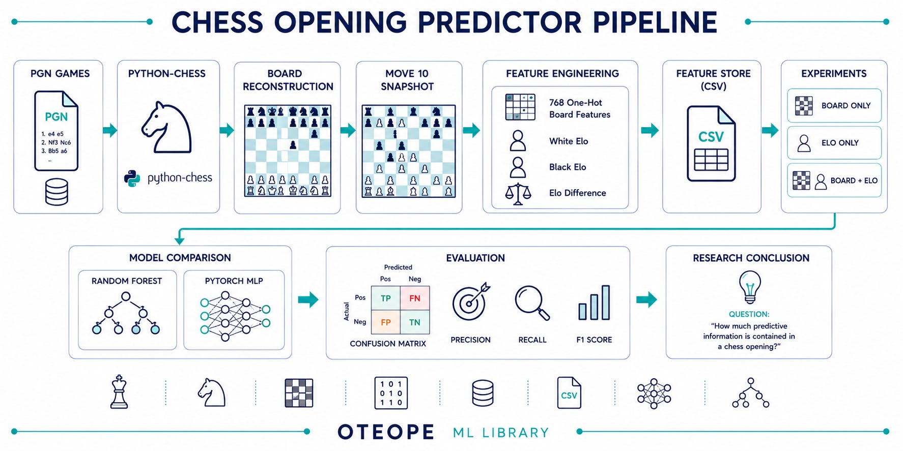
How Much Predictive Signal Is Hidden in a Chess Opening? | HackerNoon
A data-driven investigation into board geometry, player Elo, and the limits of early-game predictions.
1. Introduction: Beyond Another Stockfish Clone
How much predictive information is actually hidden in a chess opening?
While players and researchers have debated this question for years, turning it into a structured empirical study is no easy task. How do you actually measure it? In this article, you’ll discover how a well-structured machine learning pipeline can shed light on this exact question.
To be clear: this isn’t another Stockfish clone or a boring, cookie-cutter chess predictor built in a weekend. This project is a scientific investigation into position evaluation and a practical, end-to-end ML experiment.
2. The Data Pipeline: From Raw Games to a Machine Learning Dataset
Most Machine Learning projects don’t fail because of the model — they fail because of the data.
Before training a single algorithm, I needed to answer a much more practical question: where would the data come from?
Scaling from 1,400 Games to a Complete Dataset
The project started in the simplest possible way. A friend of mine, around 2000 Elo, exported his Chess.com games and sent me the PGN file. Unfortunately, the site’s export limits meant I only had about 1,400 games.
That was enough to prototype the pipeline, but nowhere near enough to train a reliable model. To increase both the size and diversity of the dataset, I combined three different sources:
- Public games from Kaggle’s Lichess dataset.
- Games downloaded from professional Chess.com accounts.
- Personal games from my friend.
For the professional dataset, I selected players with very different profiles: Magnus Carlsen, Hikaru Nakamura, Ding Liren, and Levy Rozman (GothamChess).
Interestingly, Ding Liren only had four available games through the endpoint I used. The sample was tiny, but I decided to keep it anyway.
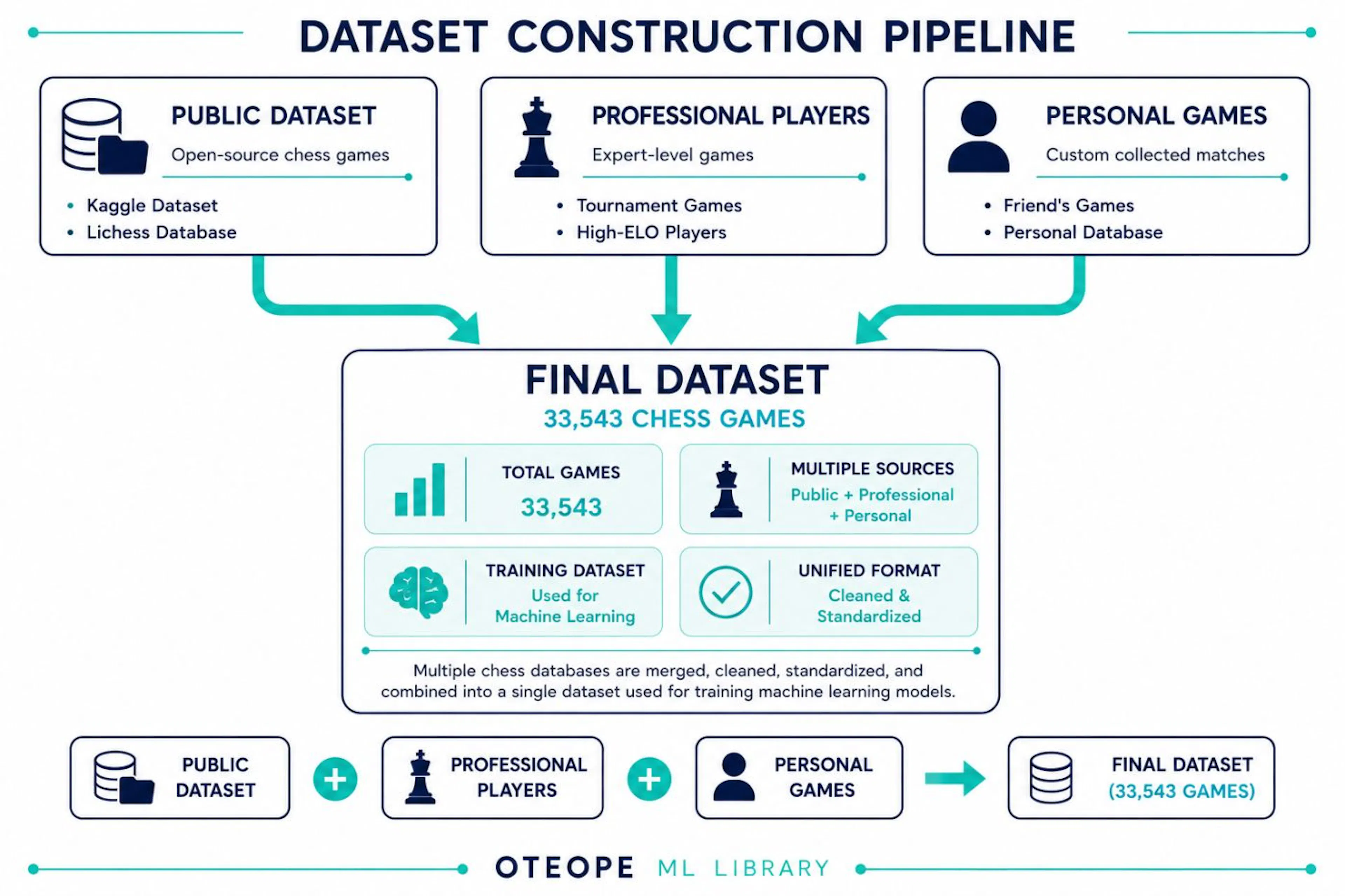 Figure 1. Overview of the three data sources used in this project: a large public dataset, professional players downloaded through the Chess.com API, and personal games collected for additional diversity.
Using python-chess, I built a parser capable of reading PGN files and stopping every game at exactly Move 10, which is the position later used by the models.
The core of the extraction pipeline simply iterates through each PGN game until the desired snapshot is reached:
import chess.pgn game = chess.pgn.read_game(pgn_file) board = game.board() for move_number, move in enumerate(game.mainline_moves(), start=1): board.push(move) if move_number == 10: break API Bottlenecks
My first idea was to retrieve games directly from the Lichess API. Although it worked, it quickly became clear that downloading and processing thousands of games this way was far slower than expected.
After several tests, I switched to Chess.com archives together with locally processed PGN files. The result was a much faster and fully reproducible pipeline.
Avoiding Dataset Bias
Another concern was preventing professional games from dominating the dataset. If one player contributed tens of thousands of games, the model could end up learning that player’s style instead of general opening patterns.
To reduce this effect, I limited every professional account to roughly 5,000 successfully processed games, producing a healthier balance between elite and intermediate chess.
Cleaning and Feature Preparation
After the extraction stage, every game went through a preprocessing pipeline. Games that ended too early or contained incomplete information were discarded, while several contextual features were added:
- White Elo
- Black Elo
- Elo Difference
The final result was a clean dataset containing 33,543 games with no missing values, ready for feature engineering and model training.
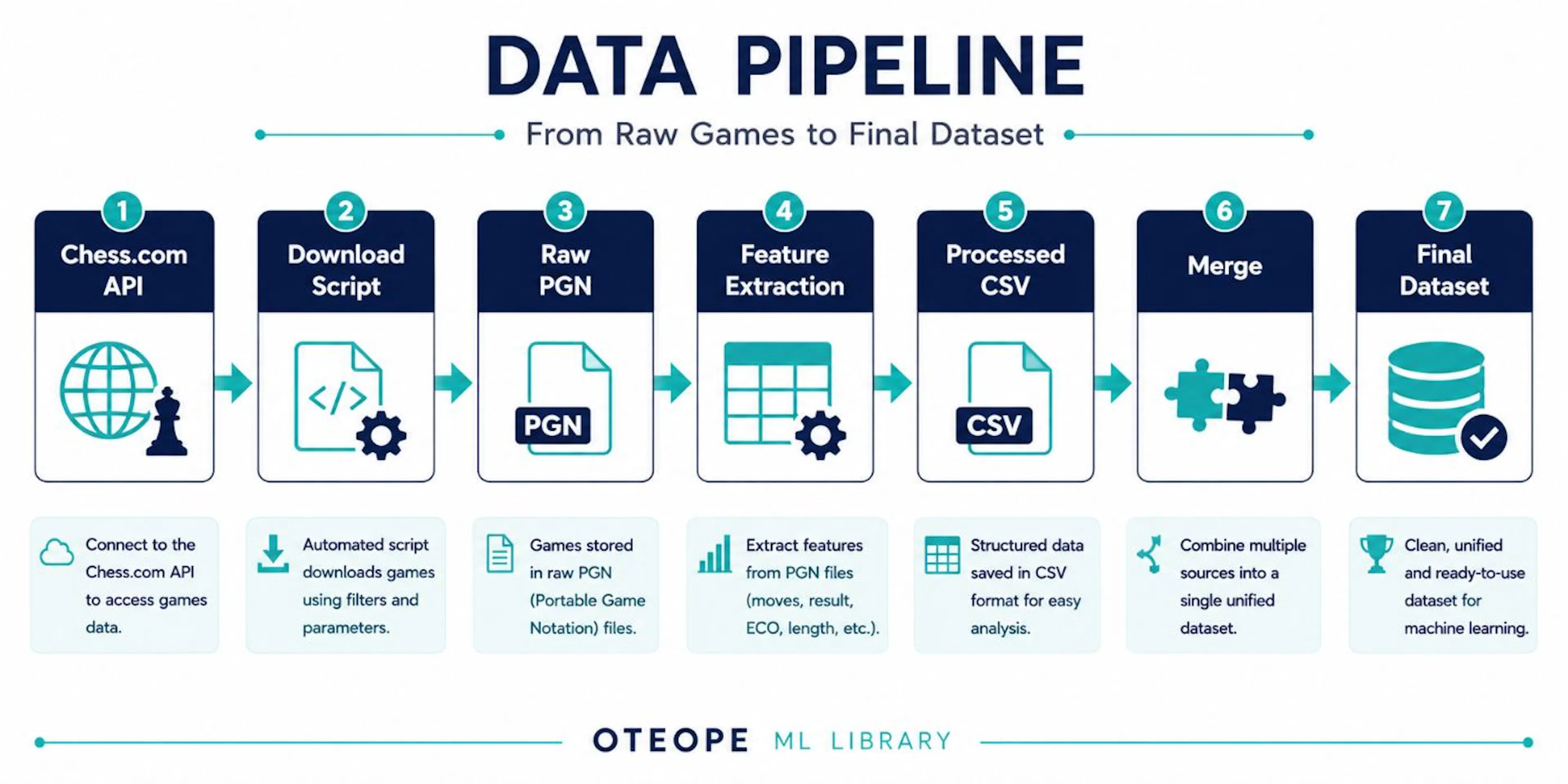 Figure 2. End-to-end data pipeline used to transform raw PGN files into a structured machine learning dataset through automated extraction, preprocessing and dataset merging.
3. Feature Engineering: Turning Chess into Numbers
Once the dataset was built, the next question became: How do you represent a chess position in a way that a machine learning model can actually understand?
Two design decisions had to be made:
- When to capture the board.
- How to encode it numerically.
Why Move 10?
Choosing the snapshot wasn’t arbitrary:
- Capturing too early: Very little information is available. Most games are still following opening theory, pieces remain undeveloped, and many positions look almost identical.
- Capturing too late: Tactical mistakes, exchanges, or decisive material advantages may have already appeared, turning the task into middlegame evaluation instead of opening prediction.
Move 10 sits in a sweet spot.
By this stage, most opening lines have either finished or started to branch into different strategic plans. Pawn structures begin to stabilize, pieces are developed, and the position already contains useful strategic information while still belonging to the opening phase.
For this reason, every game in the dataset is frozen immediately after Move 10.
Representing the Board
Machine Learning models cannot process chess boards directly. The first step was to convert every square into a categorical value representing its content:
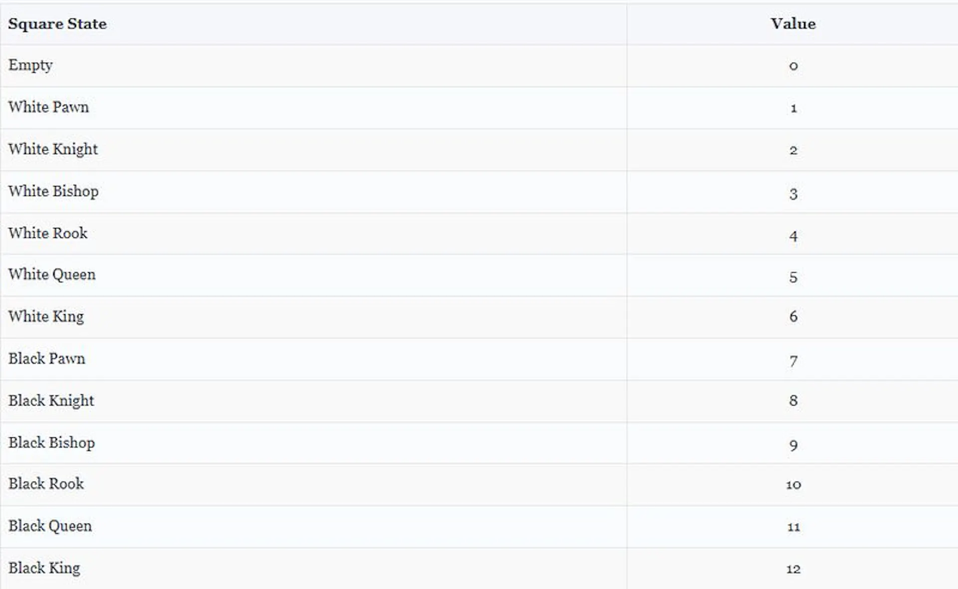
However, using these integers directly would incorrectly imply that some pieces are “larger” or “more important” simply because their IDs are higher.
To avoid introducing any artificial ordering, each square is represented using One-Hot Encoding. Rather than assigning an integer to a piece, every board position is transformed into a binary feature vector.
The final feature vector contains 771 input features, composed of:
-
768 One-Hot encoded board features (64 squares × 12 possible piece states)
-
White Elo
-
Black Elo
-
Elo Difference
Finally, the board representation is concatenated with the contextual Elo features to build the final input vector passed to every model.
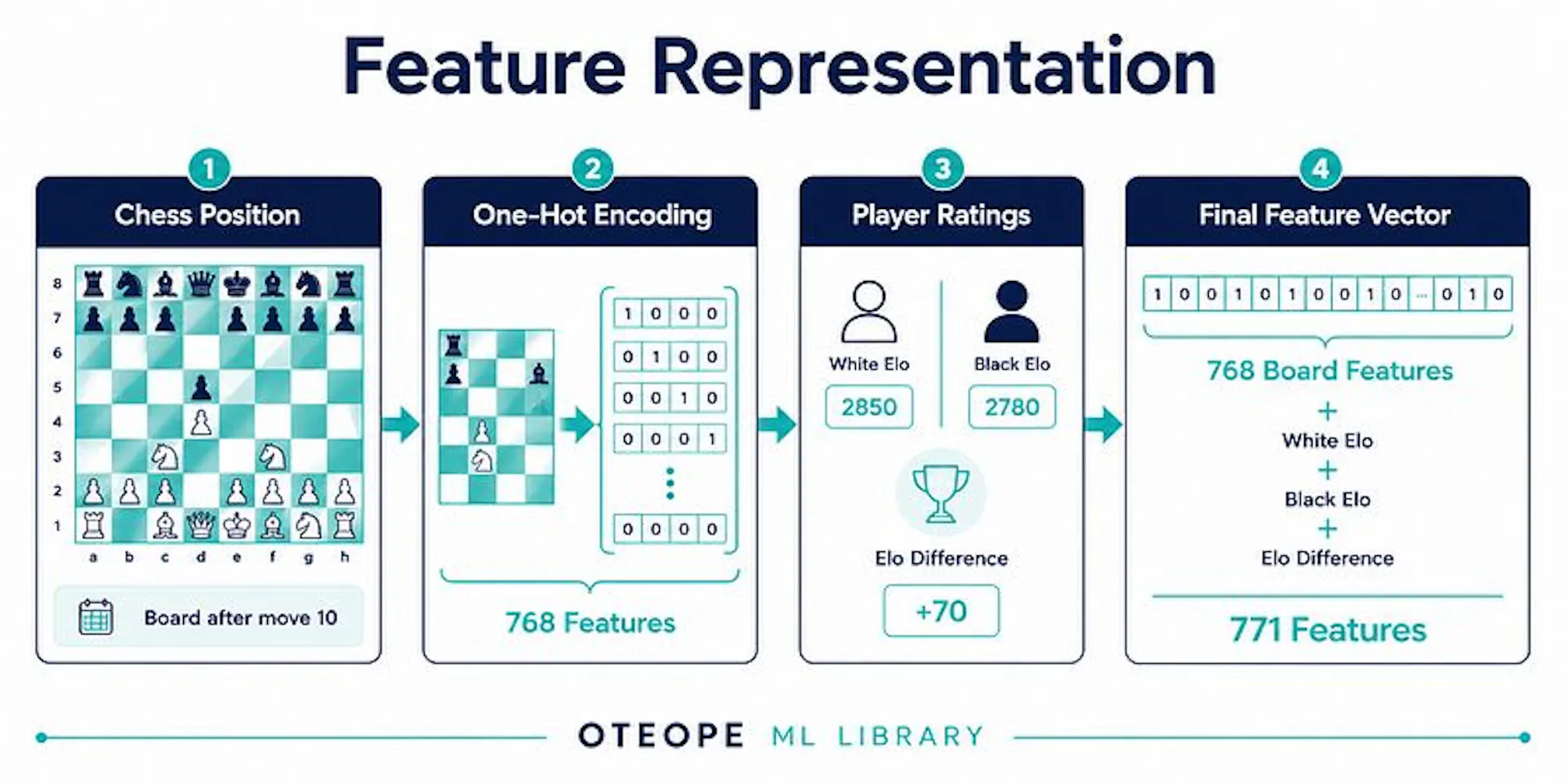 Figure 3. Feature engineering process used to convert a chess position into a numerical feature vector combining One-Hot encoded board representation with player Elo information.
features = np.concatenate([ board_vector, [white_elo, black_elo, elo_diff] ]) This representation preserves the exact board geometry while remaining suitable for both Random Forests and neural networks.
PIECE_TO_ID = { "P": 1, "N": 2, "B": 3, "R": 4, "Q": 5, "K": 6, "p": 7, "n": 8, "b": 9, "r": 10, "q": 11, "k": 12 } board_vector = [] for square in chess.SQUARES: piece = board.piece_at(square) if piece is None: board_vector.extend([0] * 12) else: one_hot = [0] * 12 one_hot[PIECE_TO_ID[piece.symbol()] - 1] = 1 board_vector.extend(one_hot) Adding Context: Player Ratings
The board alone doesn’t tell the whole story. The same position can have a very different meaning depending on who is playing it.
A slight positional advantage in the hands of a 2600-rated Grandmaster is statistically much more likely to become a win than the exact same position played by two club players.
To provide that context, three additional features were added:
- White Elo
- Black Elo
- Elo Difference
These variables allow the models to combine board geometry with player strength instead of relying exclusively on the position itself.
4. The Contenders: Random Forest vs. Multi-Layer Perceptron (MLP)
With a clean, One-Hot encoded tabular dataset ready to go, the next hurdle is algorithm selection.
Many developers fall into the “model rabbit hole,” spending months testing every algorithm under the sun. However, a strong ML engineer knows that model selection should be driven by data architecture, not hype.
I deliberately chose to benchmark two distinct paradigms:
- Random Forest Classifier (Scikit-Learn): A classic ensemble method. Despite being an older algorithm, decision tree ensembles remain among the strongest classical methods for tabular data.
- Multi-Layer Perceptron (PyTorch): A dense Feedforward Neural Network. Since MLPs are the foundational building blocks of Deep Learning, I wanted to see if deep dense layers could uncover hidden non-linear relationships in the board structure.
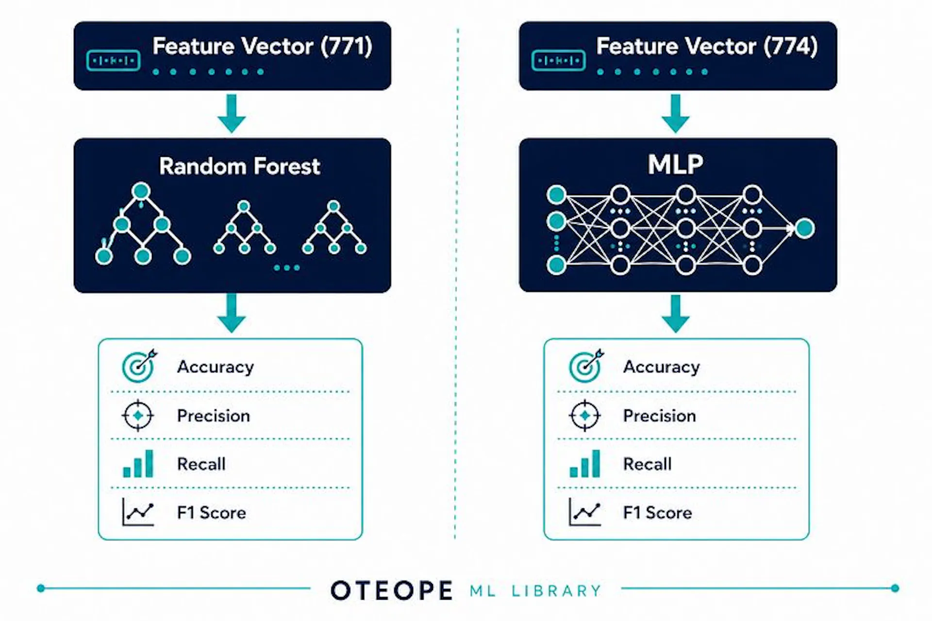 Figure 4. Comparison of the two predictive models evaluated in this study: a Random Forest classifier and a Multi-Layer Perceptron (MLP), both trained using the same feature representation and evaluation metrics.
While more specialized architectures like CNNs or XGBoost exist, the scope of this project was to prove that these baseline models can extract deep signal from chess data if the pipeline is well-engineered.
Going into the training phase, my hypothesis was clear: I expected the MLP, with its deep learning capabilities, to absolutely destroy the simpler Random Forest. The results, however, left me with a very different impression.
The final Random Forest configuration is summarized below. Most of the tuning effort focused on controlling overfitting while maintaining strong predictive performance.
rf = RandomForestClassifier( n_estimators=300, max_depth=25, min_samples_leaf=2, class_weight="balanced", random_state=42 ) rf.fit(X_train, y_train) The final MLP architecture consisted of four fully connected layers with Batch Normalization and ReLU activations.
model = nn.Sequential( nn.Linear(774, 512), nn.BatchNorm1d(512), nn.ReLU(), nn.Linear(512, 256), nn.BatchNorm1d(256), nn.ReLU(), nn.Linear(256, 128), nn.ReLU(), nn.Linear(128, 3) ) Although the architecture is relatively simple compared to modern deep learning models, it provided a solid baseline for comparing classical machine learning against neural networks on structured chess data. During experimentation for the MLP architecture, 3 auxiliary game-state indicators (active turn and castling rights) were included alongside the 771 board and Elo variables, bringing the total input dimension to 774. This minor addition helped stabilize PyTorch training without altering the core feature engineering framework.
5. Results and Discussion
Now for the moment of truth. Surprisingly, the Random Forest outperformed the Neural Network.
While the margin wasn’t massive, it completely shattered my initial assumption. For tabular representation without a spatial inductive bias (like convolutions provide), the ensemble of decision trees found direct cut-off rules much more efficiently than the dense network.
The Random Forest Reality Check
When evaluating the Random Forest, an interesting paradox emerged. The very first iteration of the model achieved the highest raw Accuracy. However, looking at the confusion matrix revealed a massive flaw: the model was completely failing to predict draws. It was over-optimizing for White and Black wins.
To fix this, rigorous regularization was applied. By aggressively tuning hyperparameters — such as capping the max_depth, tweaking min_samples_leaf, and adjusting the number of estimators—the model became much more robust. The final optimized Random Forest sacrificed a bit of overall Accuracy to achieve a much healthier generalization across all classes.
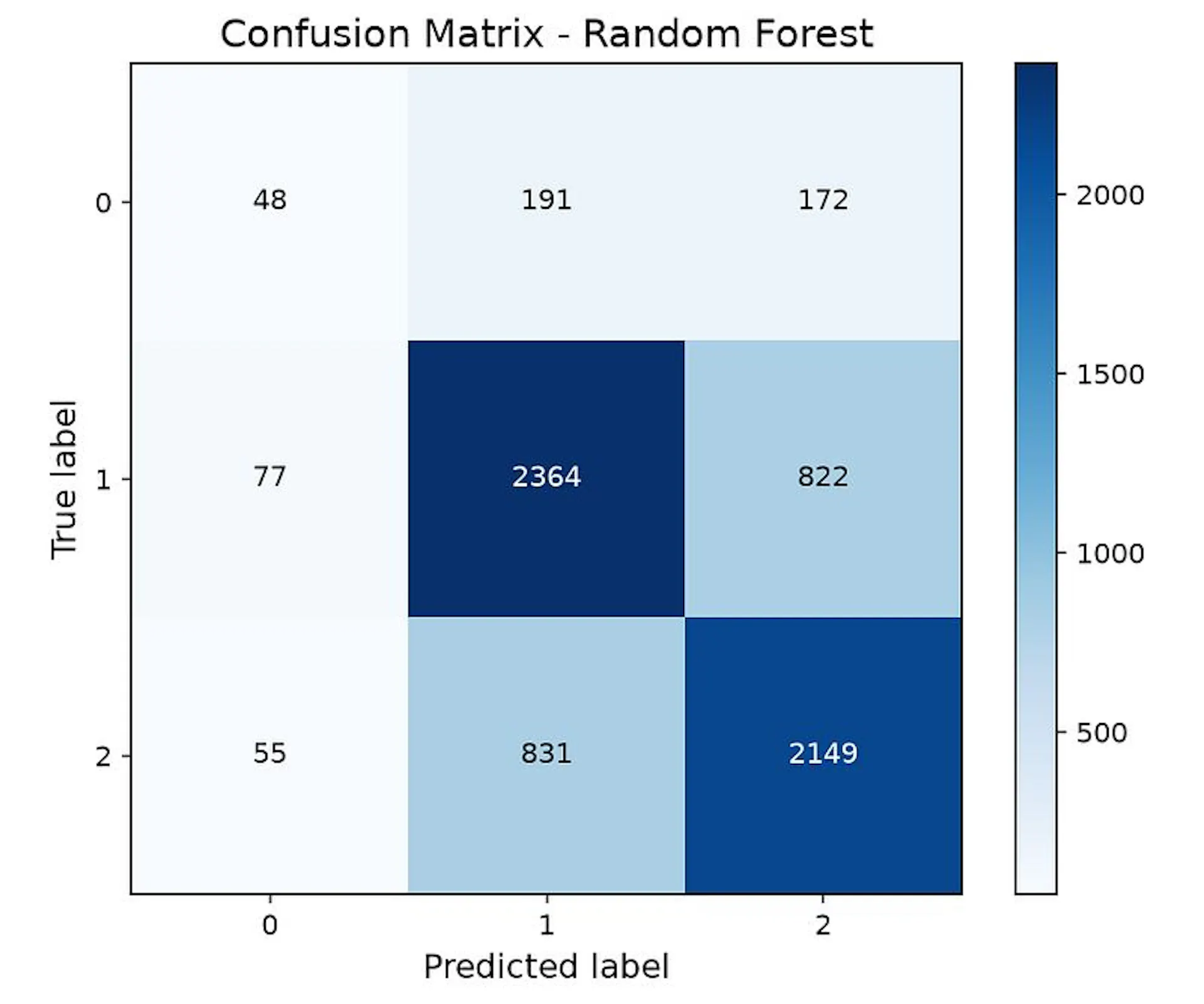 Figure 5. Confusion matrix obtained by the optimized Random Forest model on the test set.
The Deep Learning Disappointment
The MLP was the biggest disappointment of the project. In the past, I viewed Neural Networks as superpowers capable of magically transforming any data into incredible predictions. Reality hit hard.
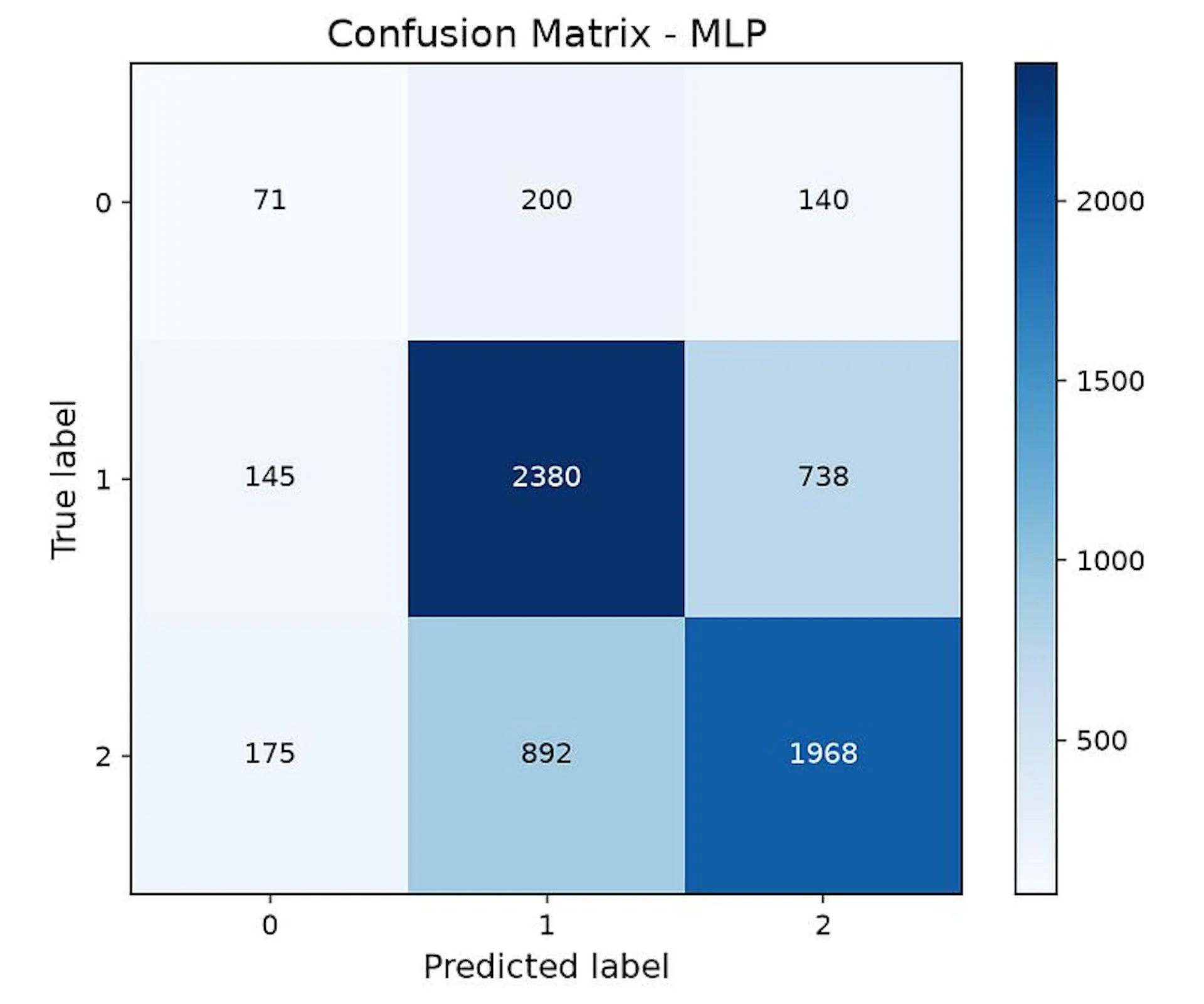 Figure 6. Confusion matrix obtained by the Multi-Layer Perceptron (MLP) on the test set.
Through iterative training, I learned two massive lessons:
- More layers do not mean better predictions. Adding depth to the MLP did not improve generalization.
- Regularization isn’t a silver bullet. We applied Dropout and Batch Normalization, and while they helped stabilize the training, they didn’t magically solve the fundamental problem: flat One-Hot encoded data is tough for dense networks to parse efficiently without spatial context. This project reminded me that adding more layers is not automatically the right solution.
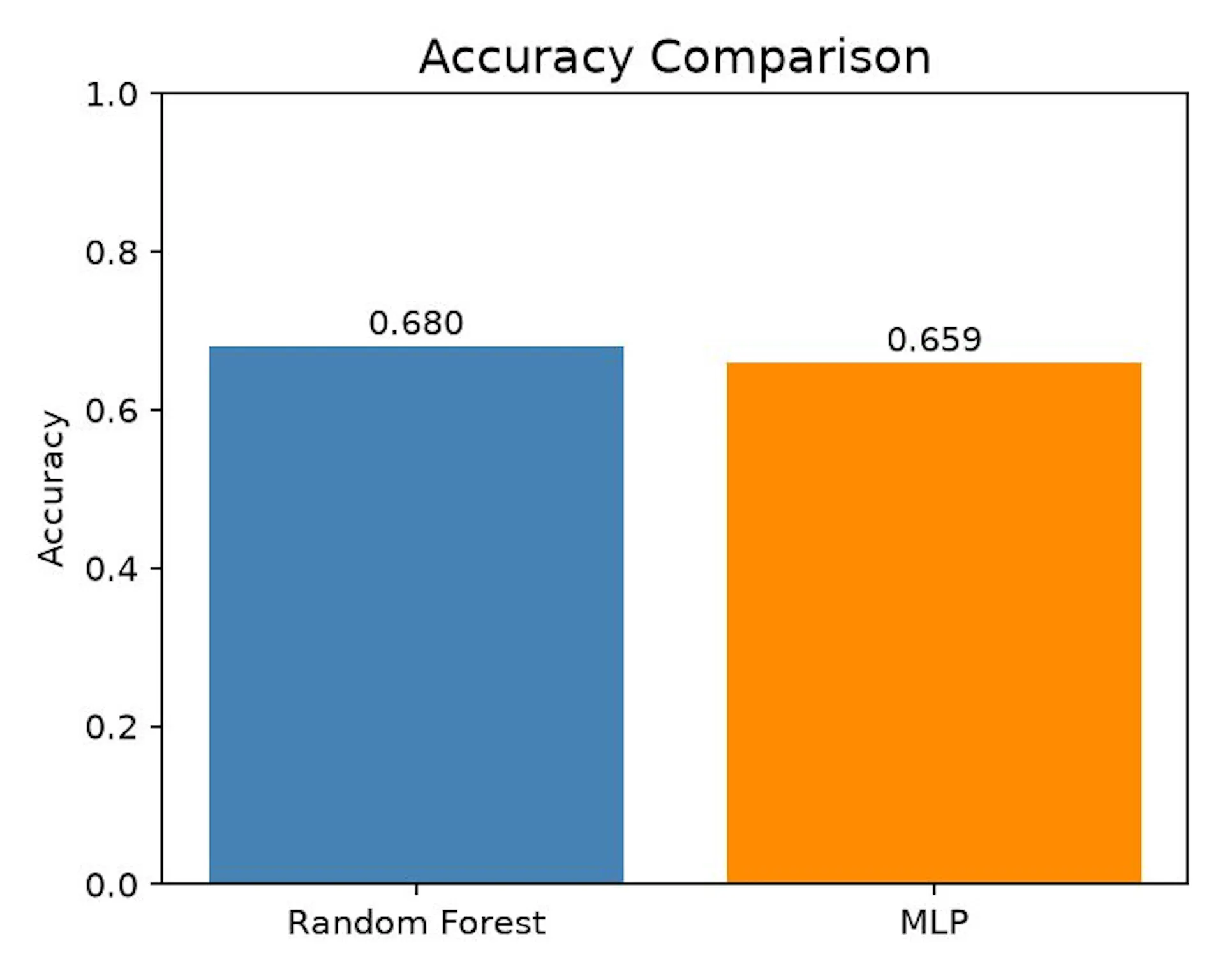 Figure 7. Performance comparison between Random Forest and MLP across the main evaluation metrics used in this project.
The Elephant in the Room: Predicting Draws
A critical factor that influenced this benchmark was severe Class Imbalance.
In professional and intermediate chess, decisive games (White/Black wins) heavily outnumber draws at Move 10. Because the dataset contained so few draw examples, neither model had enough statistical volume to learn the subtle positional nuances that lead to a peaceful handshake.
Predicting a draw purely from the opening phase is intrinsically chaotic. Even if we artificially force the models to pay attention to draws (using techniques like class_weight='balanced'), the predictive signal at Move 10 is simply too weak to confidently call a draw.
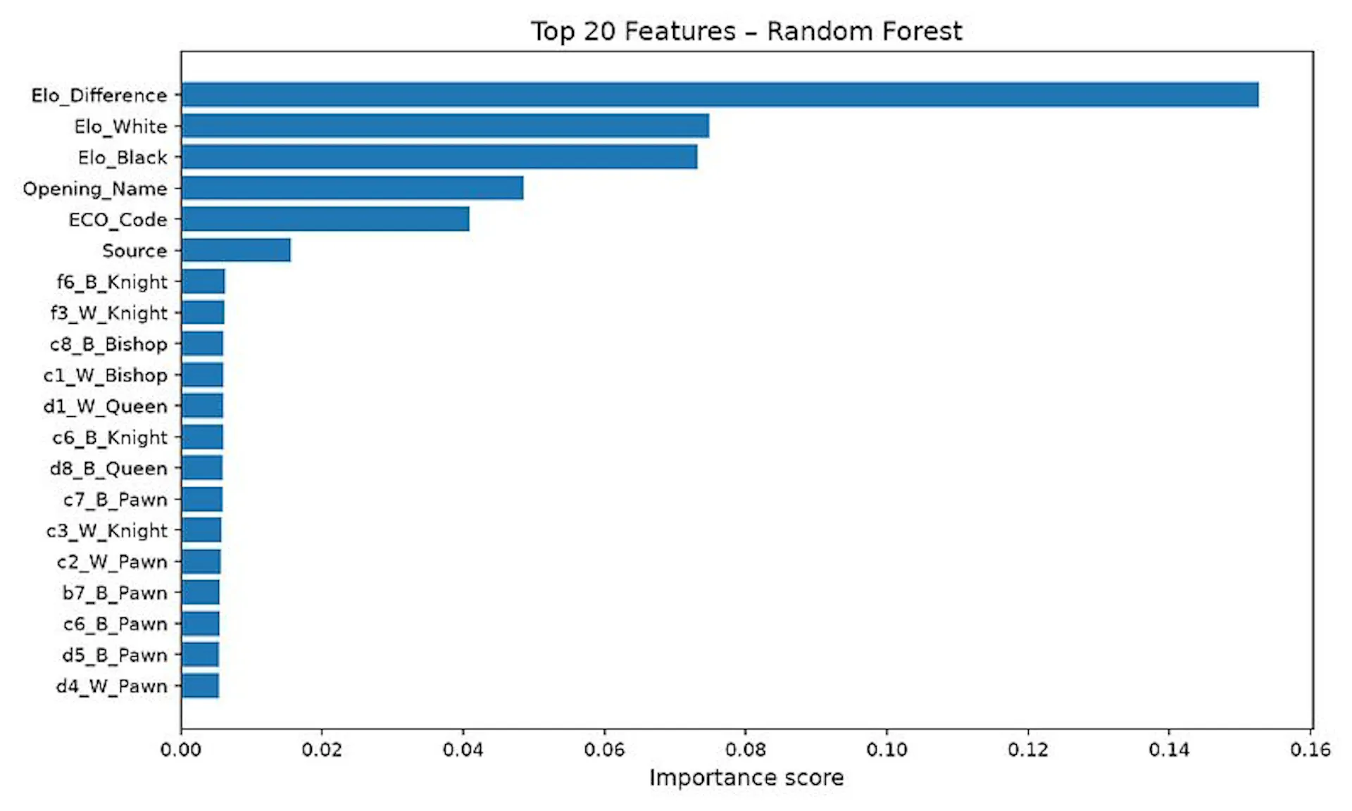 Figure 8. Top twenty most influential features according to the Random Forest feature importance analysis. Elo-related variables dominate the predictive signal, followed by opening metadata and board configuration.
6. Conclusions: What This Project Taught Me About Machine Learning
Building this project from scratch gave me a much clearer understanding of what developing a real Machine Learning pipeline actually looks like.
Before starting, I expected that training the models would be the hardest part. In reality, it wasn’t. The most difficult and time-consuming phase was data collection and preprocessing. Handling API rate limits, restructuring the extraction pipeline several times, parsing thousands of PGN files, and validating the final dataset required far more time than training any model.
One of the biggest lessons I learned is that newer or more complex models are not automatically better.
Today, generative AI can help you implement almost any Machine Learning algorithm in just a few minutes. However, understanding why an algorithm works is still essential. That mathematical intuition is what allows an ML engineer to choose the right model for a given problem instead of simply trying every architecture available.
This project also completely changed my perception of Deep Learning. I initially assumed that the MLP would easily outperform the Random Forest simply because neural networks are more powerful. Instead, the opposite happened. The Random Forest consistently achieved better results on this structured tabular dataset, reminding me that the best model always depends on the data rather than on popularity.
Finally, I learned something that every Machine Learning practitioner eventually discovers: experimentation is not wasted time. Throughout the project I tested multiple architectures, different regularization strategies, class weighting techniques and optimization methods. Many of them produced little or no improvement, but every experiment helped me understand the behaviour of the models a little better. If I had to summarize this project in one sentence, it would be this: good machine learning starts with good data, not increasingly complex models.
7. Future Work: Where This Project Could Go Next
Although the current results are encouraging, I believe there are several interesting directions that could significantly improve the project.
CNNs for Spatial Board Representation
One limitation of the current approach is the board representation itself. Flattening an 8×8 chessboard into a one-dimensional vector removes most of its spatial structure.
Representing the board as a true 8×8 matrix would allow Convolutional Neural Networks (CNNs) to better preserve local spatial relationships between pieces, potentially capturing pawn structures, diagonals, files and attack patterns much more naturally.
Sequential Models
A chess game is fundamentally a sequence of decisions rather than a single static position.
Instead of predicting the outcome from one frozen board at Move 10, a future version could model the entire sequence of opening moves using recurrent architectures or Transformer-based models. This would allow the network to learn not only the position itself but also how it was reached.
Graph Neural Networks
Another promising direction would be representing the chessboard as a graph.
Instead of treating squares independently, pieces could become graph nodes while legal moves, attacks or defensive relationships become edges. A Graph Neural Network (GNN) could then learn interactions between pieces regardless of their physical distance on the board, potentially providing a much richer representation of positional play.
Exploring Different Opening Depths
This project freezes every game after Move 10 because it provides a good balance between opening information and avoiding obvious tactical advantages.
However, it would be interesting to repeat the entire experiment using later snapshots such as Move 15 or Move 20 to investigate how predictive performance evolves as the game gradually transitions into the middlegame.
Thank you for reading!
I hope this project has shown that building a Machine Learning system involves much more than choosing a model. Data collection, preprocessing, feature engineering and experimentation all play a fundamental role in the final performance.
If you’d like to explore the implementation, inspect the data pipeline or reproduce the experiments yourself, you can find the complete source code here:
Repository
The complete implementation, together with the data pipeline and all experiments, is available on GitHub.
GitHub Repository → https://github.com/oteope/chess_opening_predictor

Related Posts